Unhiding Column A - Happy St. Patty's Day!

Happy St. Patrick's Day!!!!!!!!!!!!!

Hide and  Unhide

Unhiding a column is usually pretty easy. All you do is select the column header to the right and to the left of the hidden column and then right-click and select Unhide.

 In the example below, Column B is hidden so I selected across the Column A header and Column C header (which means that Column B was also included) and then selected Unhide from the shortcut menu.

Unhiding is a little more difficult when you have hidden Column A. To unhide Column A you need to go to the Name Box located above Column A and B and type A1.

 Then press Enter.

This forces Excel to put the cursor into cell A1. At that point, you can right-click and select Unhide. It may look like nothing happened but Excel did unhide it. Excel tends to keep the width so small that you may still not be able to actually see Column A even though it is unhidden. If that is the case, move your cursor carefully until you get the cursor to look like a 4 headed cross which will allow you to widen Column A.

Variance in a Range

Someone asked me how to find the variance of  the highest number and the lowest number in the same range of data.  The simplest way to do it is =Max(range)-Min(range).
In the simple below, I applied this formula =MAX(A3:A11)-MIN(A3:A11) so that Excel found the highest number in the range which was 90 and then subtracted it from the lowest number it found which was 5. So, we end up with a variance of 85.

Round and Rounds She Goes....

Guess how many rounding functions Excel offers............
Did you guess 10? If so, you are correct..there are at least 10.

ROUND(), ROUNDUP() and ROUNDDOWN() all round a number to the specified number of digits, either up or down depending upon the function selected. = Round() rounds up if the digit is equal to 5 or higher and rounds down if less than 5. ROUNDUP() always rounds up and I'm sure you have already guessed what ROUNDDOWN() does.

MROUND() is similar to ROUND() only it rounds to the specified multiple instead of the specified number of digits.

FLOOR() and CEILING() round to the nearest multiple. They are similar to ROUNDUP() and ROUNDDOWN() only instead of rounding to the specified number of digits, they round to the nearest multiple. You generally see FLOOR and CEILING being used in conjunction with currency- to round prices up or down.

EVEN() and ODD() round to the nearest even or odd integer.
INT() rounds down to the next lowest integer.
TRUNC() is similar to ROUNDDOWN () but rather then rounding to a specific number of digits, it simply cuts off the specified number of digits.


Below is a spreadsheet showing the results of these different rounding functions:

Click on the spreadsheet to make it larger and easier to see or to access the spreadsheet itself,  click here

Ranking a List

Rank.EQWhat do you do if you need to determine the order of your golf score or perhaps sales volume? The easiest way obviously is to sort your data in ascending or descending order but sometimes you don't have that option. If you can't reorder your data then you can use RANK().
In Excel 2010, they have renamed this function to RANK.EQ() and Microsoft recommends that you begin using it but RANK() still works.



The sytax for both RANK and RANK.EQ are:
Syntax:

• Number is the cell or number whose rank you want to find
• Ref is the array (list of numbers)
• Order is optional. The default is 0 and that means descending order

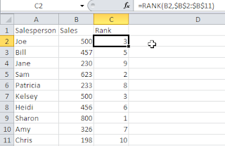
In my first example here, I used the RANK function and looked at the order of the sales in Column B. Sharon down at Row 9 has the highest sales followed by Sam at Row 5. Now the problem... Both Joe's sales and Kelsey's sales are ranked as 3 and there is nothing ranked 4th. Because there were so many complaints about this, Microsoft add two new functions in Excel 2010 - RANK.EQ and RANK.AVG.

As you can see from the illustration below, RANK.EQ  has the exact same result as RANK. Joe and Kelsey are both still ranked at 3rd and there is no 4th ranking.  Sorry, I have no clue why Microsoft would just rename a function.

Microsoft did come up with a new ranking function in Excel 2010 too. It is called RANK.AVG.

In this case, if more than one value has the same rank then the rank is averaged. So, now Joe and Kelsey are each ranked as 3.5 rather than 3 and there is still no 4th ranking.

So, RANK.EQ or RANK.AVG may work for you, particularly if you do not have values that are the same however if you wanted to do a Vlookup or an Index Match based upon the rank - you would obviously have a problem since the lookup isn't going to know that two of your values have the same ranking and that rank 4 is missing. To compensate, you can include a CountIf to identify any duplicates and get a useful ranking.

In Cell I2, the formula does not include the CountIF formula since it is the first value and there is nothing to compare it to. The formula is just =RANK.EQ(B2,$B$2:$B$11,0)

In Cell I3, I changed the formula to =RANK.EQ(B3,$B$2:$B$11,0)+COUNTIF($B$2:B2,B3) which you can then copy down.

The RANK.EQ or RANK formula assigns the rank and then the Countif looks at the cell(s) above and compares it. The CountIF returns a value of 0 if it does not find a duplicate. It assigns a value of 1 if it finds a duplicate. So, when the COUNTIF gets to row B7, it determines that value of 3 already exists in the list so its resulting answer is 1.

This formula result of 1 is added to the Rank value of 3 and Kelsey is now assigned a ranking of 4
(If Excel had  found a 2nd duplicate ranking (3 cells containing the same ranking) the CountIF formula result would be 2).

If you want a copy of this file, click here.

Also please note the use of the absolute relative references and the relative references otherwise when you copy it down, it will not work.

Extracting Different Parts of a Date

Extracting different parts of a date

This is just a quick tip that you might find useful. A lot of times, you have a column of dates and if you could easily extract the month and/or the year you would be able to sort or filter your data by it. It's really quite easy - you just use the Text function and the different date formats. I have a couple of examples below: