Creating Multiple Pivot Tables All At Once

If you are using Pivot Tables, it is extremely easy to create multiple pivot tables from your original pivot table by using the Report Filter.
The Report Filter which displays at the very top of the pivot table  is the best feature within the pivot table as it controls all the information seen in the pivot table. It also allows you to easily generate multiple pivot reports.



In the example below, Ship Via is showing as the Report Filter. Currently, I am seeing the total orders for all the ships but I can easily generate a separate pivot table for each of the individual carriers.

1. Click on a cell in the pivot table

2. Go the Options contextual ribbon





3. Select the little down arrow next to Options  (in the first group on the ribbon),

4. Select Show Report Filter Pages…..

4. Select the Report Filter that you want to view in detail. We only have one report filter here so you would select
5. Click OK




It may seem as though nothing happened however if you look down at the sheet names in your file, you will see that Excel has created worksheets for all the individual carriers. In my example, I now have a worksheets named UPS, Parcel Post, FedEx etc and when I select the sheet named FedEx I have a pivot table just showing the orders FedEx. If I click on the UPS sheet, then the pivot table displays just the order information for UPS.

Here is another quick example: If the report filter allowed you to select between 4 Salespeople, Smith, Jones, Brown and White and the Report Filter instead of displaying All was displaying Smith, you would see 3 sheets at the bottom that Excel created – Jones, Brown and White. (Jones would not display as a new separate sheet as that is already displayed on the “original worksheet”.

This can be a big timesaver.

Automatically Updating Your Pivot Table

Maybe it is a coincidence or maybe because it is because I am updating my Pivot Table EBook for Excel 2010 for CPASelfstudy.com  but I have been seeing  a lot of questions and comments regarding updating pivot tables automatically as new data is added. So, of course I thought I would talk about it here.

The good news is that in Excel 2007 and Excel 2010, it is very easy to set your data up so that Excel will automatically pull it into your existing pivot tables. The reason for this is that Excel 2007 and Excel 2010 allow you to easily format your data as a table. Once Excel considers your data a table, it automatically treats all the data as part of the table even as data is added or removed from the parameters of the table. You still need to click the Refresh button when the data changes but you don't have to change the source data location each time anymore.

Here is how to change your data into a table

• Click in the data
• Click Insert tab
• Click Table
• Verify the data range  and make sure the checkmark is in "My table has headers"
• Click OK

That's it, Excel now considers your data to be a table.  If you open your Pivot Table and re-select  your data source, the pivot table will now update as the range changes.  Now, if data is added it will automatically be incorporated into the parameters of the original source data.


By the way, another plus of turning your data into a table is that Excel automatically displays alternating row shading and AutoFilter drop down boxes for you.

 

 

Viewing the Supporting Detail behind the Pivot Table

Pivot tables are used to summarize large volumes of data however sometimes you want to see the underlying information that supports a number in the pivot table.

  The good news is that it is very easy to do - all you have to do is double-click!

Below is an example to illustrate:
I have a pivot table that is showing shipments by customers and their total order amount.

I want to see the supporting data for my customer Backpedal Cycle Shop at row 13.


When I double-click A13, the Show Detail dialog box pops up.
This dialog box allows me to specify what supporting detail I want to see.

 I selected Product Name and clicked OK.

Excel then displays the detail for Backpedal Cycle Shop's orders by Product Name.

In Excel 2010, it actually displays the supporting detail in the pivot table itself. In earlier versions, it places it on a new sheet. Notice all the detail is indented to make it easier to see.

A minus sign now appears to the left of Backpedal Cycle Shop. If you click the minus sign the detail will disappear and a plus will be display. Click again and the detail appears.

Slicers! A better way to filter Pivot Tables (Excel 2010)

If you use pivot tables, then you already know they are one of the best features in Excel. The good news is that Excel 2010 actually makes using pivot tables even better with their creation of the slicer. Sounds like a Ron Popeil commericial doesn't it?  It slices, it dices.....................

Anyway, in earlier versions of Excel, you could filter pivot tables but the field you filtering had to be in the pivot table and the drop-down box would just display the text "multiple fields" so no one at a glance knew what the heck you were filtering and displaying in your pivot table.

The slicers are essentially dialog boxes containing all the field names that remain on the screen. You select the ones you want and the data in the pivot table adjusts to what is specified.

Here are the steps

• Click in your pivot table

• Click on the contextual Options tab
• Select Insert>Slicer
• Click Insert Slicer...

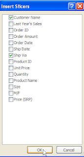
A dialog box of all the field names that comprise your data (not just the data in the current pivot table) displays

• Select your field (s)
• In this example, I selected multiple fields -Ship Via and Customer Name

• Click OK

The selected slicers display on the spreadsheet

• Click on the fields that you want to see.

 To select multiple fields in Ship Via for instance, select the first one and then hold down the control key to select the next.     

In my example, I selected Fed Ex, Parcel Post and UPS from the  Ship Via slicer and I selected the Backyard Cycle Shop as the customer I was interested in.

The pivot table now displays only data  for that one customer if one of those 3 specified carriers were used.

How cool is that.  The slicers stay there on the page and can be moved around so now you can clearly see that is being filtered and displayed in the pivot table. Think how useful this could be on a dashboard.