Determining Median and Mode

Determining the Median and Mode

Sometimes determining the average is not sufficient.
For example, if  you are analyzing departmental salaries you might want to know the median or mode of the salary levels.

=Median(data range)  internally sorts the data and  then displays the middle value. If there is an even number of values, then the two values in the middle are averaged. =Median(B2:B10)

=Mode(data range) will display the value that appears most often. =MODE(B2.B10)

This from an excerpt from my Excel CPE Course, Must Know Excel Tools and Tips for CPAs.  

TRACKING FORMULA ERRORS in SPREADSHEETS
Guest Post: J. Helstrom

Spreadsheet formula errors may cause other calculations to also yield an error message.

This is aggravating, especially if you’re working with a large worksheet.

Formula errors can be fixed -  the hard part is finding all of them.

Luckily, Excel provides a handy tool for identifying formula errors.  It’s embedded within the Find & Select icon on the Home ribbon.

Press Find & Select, then click on Go To Special…

  or press the  F5 key and then click Special....

The following dialog box appears:

Click the Formulas button and then deselect everything except the Errors check box as shown below:

Click on OK and all errors in the worksheet are now highlighted.

As an example, assume that a worksheet contains the following errors:

When Find & Select…Go To Special…Formulas…Errors is selected as shown above, the result is:

Excel has highlighted all the error messages. 

If you haven't used Go To Special before - take a look at it. You can do a lot of cool things with it such as selecting visible cells only and  it also allows you to find cells containing Conditional Formatting and Data Validations among other things.

Creating Multi-Tiered List with Data Validation and INDIRECT

I found a great tip on one of my LinkedIn Excel Discussion groups. It was how to create a multi-tiered list.

The example used was state and city.  Using a data validation in Column A to list states, the person wanted the associated cities to display in Column B.  In other words, if Cell A1 displayed Indiana then B1 should display a list of related cities. If A1 changed to Massachusetts then the list of related cities should change to reflect that.

I thought I would share this tip with you but I wanted to take it a step further so that you can see how to do this using separate sheets and not have all the data in one sheet. I also decided to do a different example so that you would see some other uses for it.

We are going to create a Product List and as different products are selected, the associated model numbers will display.

Let's go through this:

I have 2 sheets - a Summary sheet and then a Model Information sheet.
Here is the sheet named Model Info. It contains the data we are going to work with.

Here is the Summary Sheet:

Put your cursor in cell A2 and then go to the Data tab and select Data Validation.

Select List from the Allow: dropdown
Put your cursor  in the Source: dialog box and select A1:A4 on the Model Info sheet.
Click OK.






The Summary sheet now has a drop-down arrow at A2.

Click in A2 and copy that blank cell with the drop-down arrow down to A5 or A6.
Click on A2 and select the drop-down arrow and select VCR from the list we just created.

What we want to do now is set up Column B so that it will display all the models associated with whatever is displaying in Column A.

Let's go to the Model Info sheet and create a range name for all of that data.
Select A1.I14 on the Model Info sheet. 
Click on the Formulas Tab and select Create from Selection.

Make sure that there is only a checkmark in left column and click OK.
This is an easy way to create multiple range names all at once. We are telling Excel to select the Left Column which in this case are the Product Line names in Column A and create that as the range name for all of the data to the right – the model numbers. This is a lot faster than individually naming each of the ranges.

Now, let’s go back to the Summary sheet for the final steps.
Select all of  Column B (select Column header).
Select Data Validation again.

In the Allow: dialog box select List again
In the Source: dialog box, type =indirect(A1)
(make sure that it is a relative reference - not an absolute cell reference. If it an absolute, every cell will display the same contents).
 
Click OK.
 
 
 
 
Since we are referencing A1 that contains the word Product, Excel is going to give us an error message. When you see it just click Yes that we want to continue.

 
 
 
To get around the error message, you could have selected specific cells in Column B but I took the lazy way of selecting the entire column.
 
 
Click on the drop down arrow at cell B2 and you should see all the model numbers associated with the VCR product line.
Click on A3 and select another product and when you click on cell B3, you will see model numbers that are associated with that product. In my example, I selected CAM for camcorders and B3 shows all the associated model numbers.

Ranking a List

Rank.EQWhat do you do if you need to determine the order of your golf score or perhaps sales volume? The easiest way obviously is to sort your data in ascending or descending order but sometimes you don't have that option. If you can't reorder your data then you can use RANK().
In Excel 2010, they have renamed this function to RANK.EQ() and Microsoft recommends that you begin using it but RANK() still works.



The sytax for both RANK and RANK.EQ are:
Syntax:

• Number is the cell or number whose rank you want to find
• Ref is the array (list of numbers)
• Order is optional. The default is 0 and that means descending order

In my first example here, I used the RANK function and looked at the order of the sales in Column B. Sharon down at Row 9 has the highest sales followed by Sam at Row 5. Now the problem... Both Joe's sales and Kelsey's sales are ranked as 3 and there is nothing ranked 4th. Because there were so many complaints about this, Microsoft add two new functions in Excel 2010 - RANK.EQ and RANK.AVG.

As you can see from the illustration below, RANK.EQ  has the exact same result as RANK. Joe and Kelsey are both still ranked at 3rd and there is no 4th ranking.  Sorry, I have no clue why Microsoft would just rename a function.

Microsoft did come up with a new ranking function in Excel 2010 too. It is called RANK.AVG.

In this case, if more than one value has the same rank then the rank is averaged. So, now Joe and Kelsey are each ranked as 3.5 rather than 3 and there is still no 4th ranking.

So, RANK.EQ or RANK.AVG may work for you, particularly if you do not have values that are the same however if you wanted to do a Vlookup or an Index Match based upon the rank - you would obviously have a problem since the lookup isn't going to know that two of your values have the same ranking and that rank 4 is missing. To compensate, you can include a CountIf to identify any duplicates and get a useful ranking.

In Cell I2, the formula does not include the CountIF formula since it is the first value and there is nothing to compare it to. The formula is just =RANK.EQ(B2,$B$2:$B$11,0)

In Cell I3, I changed the formula to =RANK.EQ(B3,$B$2:$B$11,0)+COUNTIF($B$2:B2,B3) which you can then copy down.

The RANK.EQ or RANK formula assigns the rank and then the Countif looks at the cell(s) above and compares it. The CountIF returns a value of 0 if it does not find a duplicate. It assigns a value of 1 if it finds a duplicate. So, when the COUNTIF gets to row B7, it determines that value of 3 already exists in the list so its resulting answer is 1.

This formula result of 1 is added to the Rank value of 3 and Kelsey is now assigned a ranking of 4
(If Excel had  found a 2nd duplicate ranking (3 cells containing the same ranking) the CountIF formula result would be 2).

If you want a copy of this file, click here.

Also please note the use of the absolute relative references and the relative references otherwise when you copy it down, it will not work.

Excel Arrays - Audit Plan Uses

I hope that everyone had a great Labor Day.
We went up to Chicago and had a great time at the Field Museum and shopping as well as eating at some great places. The weather was perfect.
I've been busy redesigning and reformatting CPASelfstudy.com to make it easier to navigate so I have not put a lot of time into this blog lately however that should change shortly.

I did want to mention that the Missouri CPA Society published our article on Incorporating Excel Arrays into Your Audit Plan as that may be of interest to you. They have an online version of  The Asset that can now be accessed  -  http://theasset.dirxion.com/WebProject.asp?BookCode=jul10flx&from=2

INDIRECT FUNCTION

The INDIRECT function is cool. When you first look at it, you wonder what the heck you can do with it and then all of a sudden you realize that you have a lot of applications for it.
The INDIRECT function accepts a text string as an argument and then evaluates the text string to determine the relevant cell or range reference. What does that mean?
Let's start with a basic example:


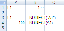
Based on the Excel spreadsheet screenshot:
=Indirect(”A1") Returns the contents of the referenced cell which is B1

=Indirect(A1) Returns the actual contents of the referenced cell. Excel sees that cell A1 contains the cell reference B1 and goes and returns the value in B1 which is 100.
If cell A1 had contained text such as CPA, then CPA would have been returned if quotes had been used.
However, if quotes were not used you would see a #REF! Error since there is no cell reference called CPA.

Okay, so what can you really do with this? Does anyone have an Excel workbook that has a sheet for each month and a summary sheet that displays key calculations for the current month? If not, perhaps you have a file contains sheets by brand or product line and then a summary sheet? If so then you probably spend a lot of time linking or copying and pasting. Using the Indirect function will save you time and allow you to more time to analyze the data.


In the example below, I have a summary sheet that tracks the current month volume in both dollars.

The supporting sheets with the store information are labeled by month - Jan, Feb and March.

 Instead of linking or pasting numbers into summary sheet cells B6 each month I can automate the process by using the Indirect function. Notice that cell B4 is the cell showing the month’s key values that I am displaying. In this case January.

 The formula I use to retrieve the total shipment dollars shipped in January is

This formula tells Excel go look at cell B4 and to find the cell or range reference found there. In this case Excel looks for JAN which is a sheet name. The ampersand joins the month name with the cell reference of G19. Excel goes to the January sheet and returns the value found in G19 to this summary sheet. If I wanted to see the value of G19 on the February sheet all I have to do is change the name in B4 to Feb to match the name of the actual sheet.

Excel goes over to the Jan sheet and then retrieves the value of 2,556,375 at cell G19 and returns it to the summary sheet.







This example was a bit simple – what happens if every month has a different number of rows or isn’t nicely totaled? If the column had not been totaled I could have used a formula such as this

or if you had no idea how many rows were being populated you could have substituted G:G for G1:G40.
To make it more efficient, use a data validation drop-down list of months in B4.

Frequency Distribution

I hope you all are enjoying this great weather. I've been working away preparing for a couple of seminars that I am doing in May and I have to tell you I've been having a blast learning all kinds of new tricks and tips that I will be sharing shortly with you. 

Today, I thought I would talk about the Frequency functions. This was quite useful to me when I taught at Butler. For all you of you instead of grades- consider using it to track warranty information or perhaps returns or HR data such as salary levels in your organization. If you think about it, I am sure you will find a couple of uses for this.

Frequency Distributions


A frequency distribution allows you to measure performance of one item against others. A good example would be a comparison of students in a class and the grade category that they fall into. Again, consider tracking returns of an item by color or even item number. Other possibililies include a breakdown of prices for a product line or even ages or education of your workforce.
A frequency distribution is a table where data in a spreadsheet is counted into bins. It is a good habit  double check your calculation - to verify that the number of items in your input range equals the number of observations in your answer. Use a COUNT function on the input range and the sum function on your answer.

To create a frequency distribution

1. Create a set of numbers to use as bins. Keeping with our grading metaphor, you may want to have five (5) bins such as the following: 100, 89, 79, 69 and 59.

In our case, we are asking Excel to group grades so that we can see the number who earned a grade between 100 and 90 as one category (the A group), those who earned a grade between 80 and 89 (the B group) etc. all the way to a count of those who earned a grade between 0 and 59.

The bins created are in Column F. The description was added in Column D and E is solely for clarification and documentation and is not used in the calculation.

2. Select the cells where you want your answer to go. In this case, select G2.G6.

3. Type = Frequency (and then select the input range. In this case you would select C2.C11.

4. Type in a comma and then select your bin range. In this case F2.F6.

5. Type a closing parenthesis. Your formula should look like =frequency (c2.c11, f2.f6)

6. Now the important part - press CTRL+SHIFT+ENTER. The resulting frequency distribution should appear and resemble Column G. The resulting formula should look like {=frequency (c2.c11, f2.f6)}

So, what does this tell you? It tells you that in the A bin which are grades between 90 to 100 (inclusive), 6 people fell into that category whereas only 2 people ended up in the C category which was from 70 to 79 inclusive.
A couple of comments:
Excel puts the brackets around the formula to show that it is an array. If at step 2, you only selected G2 and after going through the other steps, you copied the formula down- the answer would be wrong, Because this is essentially an array formula, you need to select all the cells G2.G6 at one time for this to work.

Also, bins must be numeric. In the example below, I want to figure out how many people have less than a high school education but my data and the bins must be numeric. Again, the description is purely for the user- it is not used in the calculation. As mentioned above, it is a good idea to sum your Frequency and then count your observations to make sure that the number are the same.  In the example below, my frequencies total 40. If I counted the number of people in my data, it should total 40 people otherwise there is a problem somewhere.

USING IF and ROUND Functions to Check Balances

CHECKING TO SEE IF YOU ARE IN BALANCE
This is a handy formula to double-check your balance sheet with:


It is often easier to type in the TRUE and FALSE components first

=IF(ROUND(C4,0)=ROUND(C6,0),"in balance","out of balance")

You have to round both cell references….

Once you have done this, if you change c6 to 99.5, C10 will display In Balance.

Tip: Always test both the true and the false components. Just because one works - that doesn't mean the other does.

I love to use Data Validation to create dropdown lists - particularly when working with Vlookups but I found it irritating that my source list had to be on the same sheet.  After being extremely lazy I finally got around to looking for a work-around and found one at Contextures.com. 

1. Create your list
2. Range Name it - (Select your data, click in the Name Box and type a name and then press Enter)

In this example, I selected my data and created a range name called product.The Name Box is directly above column A.

• Select a sheet and cell where you want the drop-down list to appear.
• Select the Data tab
• Select Data Validation
  
  Select List from the Allow: drop-down
  In the Source: section, type = product
• Click OK

  

Click on the drop-down and see the list you created.

Cumulative Totals

Sometimes it is the easy stuff that escapes us.
Below is a screenshot showing how to create a cumulative total.

In the example below, I want to create a Running Total and track my T-Shirt Returns.

• Click in cell D3 and type =SUM($B$3.B3)
• Press Enter
• Copy the formula down.

Why this works:                                                                            
The $B$3 creates an absolute cell reference so that as the formula is copied down, it always goes back and refers to B3.
If you click in cell D4, after you create the formula, you would see that the formula has now changed to
=SUM($B$3:B4). The first cell reference is an absolute and anchors the cell reference in place but the second cell reference moves down a row.
The formula at D15 would of course read as =SUM($B$3:B15).

Smart Tables in Excel 2007

Excel 2007 offers a wonderful feature that not many people are aware of.  It is called a Smart Table and, in my mind, is basically an advanced version of Excel 2003’s List feature.

Excel considers a list or table to consist of data that is adjacent and does not contain a totally empty column or a totally empty row.
With the Table feature, you can have new data formatted as you enter it, shade alternate rows, instantly sum up the right column and quickly name the table.



The most exciting feature however is that tables are dynamic. As you add or delete data, Excel automatically updates and formats the table. So, what does this really mean for you? It means that if you base a chart, a pivot table or a formula on a table, as data changes in the table, it will automatically update the chart or whatever it is based on. This ensures that you are working with the most current data.


CREATE A TABLE
To create an Excel table

• Type your data into the worksheet as you normally would
• Make sure that you include column headings
• Do not leave any empty rows or columns
• Click in the data and press CTRL+T.

The Create Table dialog box will pop up so that you can double-check the data range and to ensure there is a checkmark in My Table has headers.

• Click OK.

The table feature automatically bands and shades every second row and it applies filter arrows to the column headings. A definite timesaver.
 

 
 
 
 
 
When the table is created, a contextual toolbar also appears.
It allows you, among other things, to quickly sum a column, name the table, change formatting styles as well as remove duplicates.
 
 

Adding data into the spreadsheet is not any different than what you have done before – you simply select a cell in the row immediately below the last row and type the value in.

-If you enter a formula in the adjacent column, Excel will automatically copy it down the entire table and format it.
-If you enter data in the adjacent row, Excel will automatically format it so that it matches the table.


To me, the exciting part of the table is that when you add the total row, Excel automatically calculates the values in the rightmost column. You can change that summary operation or add a total to another column easily.



To Create a Total Row
-Make sure your cursor is in the table
-Click on the Design tab under the new Table Tools tab
-Click Total Row

The last row of your total now displays the sum of the right most column.

Duplicates

Great game although The WHO vocals and the ads were a bit of a disappointment.

DUPLICATE VALUES

I've had a number of emails and conversations lately about identifying duplicate values.
Using Conditional Formatting in Excel 2007 makes it relatively easy but not everyone has Excel 2007.
Let's start with Excel 2003:

Let's say that you have a column of numbers in B4:B16 and you want to identify duplicates.

Method 1:
Sort - Easy but sometimes you can't or don't want to manipulate your data.

Method 2: Click in cell C4 and type

and then copy it down.

You will have a column of TRUE and FALSE.  You can manually delete them or highlight them. The problem with this method is that Excel labels both numbers are TRUE - there is no differentiation between the original and the duplicate.

Method 3:  A Better Alternative
To get around this, try =IF(ISNUMBER(MATCH(B4,$B$3:B$3,0)),"Duplicate","Unique").
This will label the original as Unique but any other instances will be labeled as a Duplicate.

Method 4: This method is actually available in Excel 2003 and Excel 2007.
You can use the Advanced Filter function under the Data menu or tab and select Unique Only.
To be honest, I have mixed results with this so double-check your answer.

Select the column of numbers and then go to the Data tab or menu and select Advanced Filter.
Click copy to another location
Enter a cell to Copy To:
Put a checkmark in Unique Records Only
Click OK.

Well, it's getting late. Tomorrow I'll talk about how to identify Duplicates in Excel 2007.