Custom Formats

MORE CUSTOM FORMATS
 

Wow... I am on a roll here........

Another useful format that some people just love is #,####,

This format takes a longer number and essentially truncates it for you so that you do not see the thousands. Excel still reads it as the longer number but you don't see it- even if I do calculations unless you re-format it.

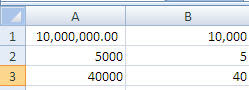
Column A shows the actual number but when copied that number into Column B and then applied the custom format #,####, it redisplayed the shortened number. So, if you don't like dealing with a lot of extraneous zeroes, take a look at this format. Although you can change the display units in a chart itself, this is another way to show simpler units on a chart you are presenting.

• Right-click on the cell(s)
• Select Format Cells
• Under Category, select Custom Formats
• Enter #,####, in the Type
• Click OK

The # tells Excel it is a number - don't forget that last comma... that's important as that is telling Excel that there are additional numbers after that but not to display them.

Keeping Leading Zeroes

LEADING ZEROES


Excel drops leading zeroes which can be a problem sometimes when you want to sort invocie numbers, account numbers or zip codes. If you want Excel to keep the leading zeroes then you need to create a custom format.

• Select the range you want to format


• Right-click and select Format Cells


• Select the Number tab


• Under Category, select Custom


• Enter the number of zeroes that your longest entry will have
  (In my example, I said 5)

• Click OK.

If you are just working with zipcodes, an little bit easier method is to select Special under Category and then select Zipcode. (Social security and telephone formats are also there.)

Find the Numbers

I'm not a "huge" football fan but What a Weekend... The Colts WON! And then of course I had to watch Minnesota and the Saints. Imagine... getting to the superbowl for the first time ever based on a field goal!

Okay... back to work. I wanted to share a tip that one of my customers emailed me. I thought you might find it useful. I call it FIND THE NUMBERS.

If you have a spreadsheet with numbers and formulas and you need to update certain "input" numbers each month and

1) you want to make sure that they are all updated
and
2) you don't want to waste time clicking on a cell only to discover it is a formula or worse yet- overwrite it in error

then this tip is for you.

• Open the spreadsheet
• Go to Edit >Goto Special if you have Excel 2003 or go to Find & Select >Go to Special if you have Excel 2007
• In the dialog box, put a checkmark in constants and one in numbers

• Click OK - Excel then selects just the cells that contain numbers - the Input cells you need to change
• Click the fill button (paint can) and apply a color or change their font color.
• As you update and change the number, remove the color formatting you applied.

By the end of the month, all the colors should be gone and you can be confident that your spreadsheet is up to date.

Nice tip Chris. Thanks.

Additional Comment Added : 1/26/10

If you have Excel 2007, you can do this even a little bit faster. Click on Find and Select and click on Constants. It will select all the constants. Apply a color such as light blue or green and you are done.

If you have a tip to share, drop me a line at patricia@cpaselfstudy.com

Using Arrays to Add Columns Containing Error Messages

I wanted to finish up my discussion of the other day - how to calculate columns containing error messages and also introduce you to Arrays. Arrays are very interesting and I think I will spend some time next week talking about them. They are extremely powerful.


This is a totally different approach from my last post which showed you how to use SUMIF if you wanted to add up a column of numbers with errors.


This approach uses an array to replace all the error messages with zeroes. Here we telling Excel to test for any errors and replace them with zeroes and to then sum the column.
In cell B8, I typed =SUM(ISERROR(B2:B7),0,B2:B7)) and then pressed Control+Shift +Enter at the same time.

The key thing to remember about arrays is that after you create the formula, you must press Control+Shift+Enter instead of just pressing enter. The 3 keystrokes tell Excel that it is an array and that all the cells are treated as a single block of cells and is depicted by the { } marks you see around the formula.
Obviously you would not use a 0 if you were trying to average the column. To get around that you could use " " to put blanks in the cells with errors.

If you are interested in arrays, you may want to check out my Arrays- A Powerful Tool course (If you are not a CPA and/or don't care about the CPE, just the Ebook is available for purchase on this site- in the far right column).
It walks you through how to put arrays together step-by-step.
Have fun and have a great weekend because... hey- it's Friday.

Summing a Column with Error Messages

I received a number of emails from people who read my last newsletter about my tip on summing a column containing error messages so I thought I would share it here with you.

SUMMING A COLUMN CONTAINING ERROR MESSAGES
If you don't already know how to do this, then this should make your year because everyone runs into it at some point.
In Excel 2003, you can use the SumIF function to tell Excel to sum all the cells in a column if they are greater than 0. By doing this, Excel will ignore any error messages, such as #N/A and DIV!0 in the column.
In the example, below, I am adding up column B and telling Excel to sum the numbers if they are greater then 0.

What to do if you have negative and positive numbers in the column? Simply add another SUMIF that tells Excel to add just negative numbers.

As with everything, there is more than one way to do this. A more elegant way is to use an array and I will talk about that tomorrow.

Have a great day and keep looking... the sun is out there somewhere