Setting up Ringtones for a Contact on your Iphone

Setting Up Different Ringtones on IPhone

You can  set up different ringtones, text tones and even different vibrations for specific people on your Iphone. This can be very useful if you want to be able to identify certain calls but you cannot immediately access your phone.

Here are the steps.

Tap the Contacts icon on the Home screen.
Select the person you want to assign a specific ringtone.
 Once you have their  page open, click on Edit ( in the top right hand corner). 
Scroll down to Ringtone; it should be set to “Default”. Click the arrow (chevron) to the right of  “Default” and select a new sound. 
When you select a new sound it will play it for you so that you can hear what it sounds like. If you don’t like it then try another one ringtone. That's it... 

This is very useful if you have kids  and you may also find it useful if you have a bothersome boss or employee :)

Hide and Seek - Column A

Unhiding a column or a columns in a worksheet is generally pretty easy.  For example, to unhide columns  C and D, simply select the  Column B header and drag across and select the Column E header (This in effect is selecting Column C and D) and then right-click and select Unhide.

Now, Column A however can be a different story since there is no column before it to select.

The easiest way to unhide Column A is to go to the Name box and type in A1 and press Enter.

Excel will move your cursor to cell A1 even though you can’t see it. 

You can then go to Format>Cells and go to Visibility>Hide and Unhide and then select Unhide Column.

I ran into a situation  yesterday where I could not get this to work. However, by selecting the entire worksheet and copying it to a new sheet all my hidden columns displayed!
To select an entire worksheet click on the  header located under the Name Box (above  row 1 and to the left of Column A)

Selecting Non- Contiguous Cells

CTRL Key

I was talking to someone the other day who had been using Excel for years but was unaware of how to select non-contiguous cells so I thought I would explain it in case you were interested. It is extremely easy.

• You select the first cell or range of cells that way you normally would.
• Then you hold down the CTRL key and select the next cell or range of cells.
• If you have another row select it (still holding down the CTRL key)
• Deselect the CTRL key when you have finished.

Yup.. that is all there is to it.

So, what can you do with this knowledge?

• Well, I love to you use this when charting.Just select the non-contiguous ranges of data you want to chart and then click Insert and select your chart type. Deselect the CTRL key.

• This is also useful if you want to format the top and bottom row of your P&L as currency. No point in selecting the top row and formatting it and then moving to the bottom row and formatting. Instead select the top row, hold down the CTRL key and select the bottom row and then apply the formatting. When finished just deselect the CTRL key.

• This also works if you have a couple of non-contiguous columns that you need to sum. Just select the first column, hold down the CTRL key and select the next column and then the next column and the next column etc. Click the AutoSum icon and all the columns will display totals.

Protect Your Workbook Structure

Protect Your Work

If you share workbooks with others then I am sure you have experienced someone inserting or deleting a sheet and totally messing up your work. Or, that helpful person who renames the sheets for you??

Anyway, in addition to protecting the cells in the sheet which I have covered in other blogs, today I want to talk about protecting your workbook's structure. It is easy to do and you will wish that you knew about this a long time ago.
These steps pertain to the entire workbook - not just a worksheet.

• Click Review. 
• Select  Protect Workbook which is located in the Changes grou.p
• Select Structure Option in the Protect Workbook dialog box.
• 4. Click OK.

If you right-click on a sheet name after doing these steps, you will see that you can no longer delete, insert or rename a sheet. In addition, you cannot change its color or hide or unhide the sheet.

If you select Windows, you can prevent users from changing the size or position of worksheet windows.



This tip is very useful if you are linking together several spreadsheets maintained by others.

TRACKING FORMULA ERRORS in SPREADSHEETS
Guest Post: J. Helstrom

Spreadsheet formula errors may cause other calculations to also yield an error message.

This is aggravating, especially if you’re working with a large worksheet.

Formula errors can be fixed -  the hard part is finding all of them.

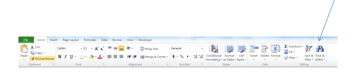
Luckily, Excel provides a handy tool for identifying formula errors.  It’s embedded within the Find & Select icon on the Home ribbon.

Press Find & Select, then click on Go To Special…

  or press the  F5 key and then click Special....

The following dialog box appears:

Click the Formulas button and then deselect everything except the Errors check box as shown below:

Click on OK and all errors in the worksheet are now highlighted.

As an example, assume that a worksheet contains the following errors:

When Find & Select…Go To Special…Formulas…Errors is selected as shown above, the result is:

Excel has highlighted all the error messages. 

If you haven't used Go To Special before - take a look at it. You can do a lot of cool things with it such as selecting visible cells only and  it also allows you to find cells containing Conditional Formatting and Data Validations among other things.