Best Microsoft Excel Bloggers

Tuesday, March 8, 2011

Round and Rounds She Goes....

Guess how many rounding functions Excel offers............
Did you guess 10? If so, you are correct..there are at least 10.


ROUND(), ROUNDUP() and ROUNDDOWN() all round a number to the specified number of digits, either up or down depending upon the function selected. = Round() rounds up if the digit is equal to 5 or higher and rounds down if less than 5. ROUNDUP() always rounds up and I'm sure you have already guessed what ROUNDDOWN() does.
MROUND() is similar to ROUND() only it rounds to the specified multiple instead of the specified number of digits.

FLOOR() and CEILING() round to the nearest multiple. They are similar to ROUNDUP() and ROUNDDOWN() only instead of rounding to the specified number of digits, they round to the nearest multiple. You generally see FLOOR and CEILING being used in conjunction with currency- to round prices up or down.

EVEN() and ODD() round to the nearest even or odd integer.
INT() rounds down to the next lowest integer.
TRUNC() is similar to ROUNDDOWN () but rather then rounding to a specific number of digits, it simply cuts off the specified number of digits.


Below is a spreadsheet showing the results of these different rounding functions:

Click on the spreadsheet to make it larger and easier to see or to access the spreadsheet itself,  click here

Monday, February 21, 2011

Ranking a List

Rank.EQWhat do you do if you need to determine the order of your golf score or perhaps sales volume? The easiest way obviously is to sort your data in ascending or descending order but sometimes you don't have that option. If you can't reorder your data then you can use RANK().
In Excel 2010, they have renamed this function to RANK.EQ() and Microsoft recommends that you begin using it but RANK() still works.


The sytax for both RANK and RANK.EQ are:
Syntax:
  • Number is the cell or number whose rank you want to find
  • Ref is the array (list of numbers)
  • Order is optional. The default is 0 and that means descending order
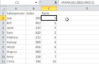

In my first example here, I used the RANK function and looked at the order of the sales in Column B. Sharon down at Row 9 has the highest sales followed by Sam at Row 5. Now the problem... Both Joe's sales and Kelsey's sales are ranked as 3 and there is nothing ranked 4th. Because there were so many complaints about this, Microsoft add two new functions in Excel 2010 - RANK.EQ and RANK.AVG.
As you can see from the illustration below, RANK.EQ  has the exact same result as RANK. Joe and Kelsey are both still ranked at 3rd and there is no 4th ranking.  Sorry, I have no clue why Microsoft would just rename a function.

Microsoft did come up with a new ranking function in Excel 2010 too. It is called RANK.AVG.
In this case, if more than one value has the same rank then the rank is averaged. So, now Joe and Kelsey are each ranked as 3.5 rather than 3 and there is still no 4th ranking.
So, RANK.EQ or RANK.AVG may work for you, particularly if you do not have values that are the same however if you wanted to do a Vlookup or an Index Match based upon the rank - you would obviously have a problem since the lookup isn't going to know that two of your values have the same ranking and that rank 4 is missing. To compensate, you can include a CountIf to identify any duplicates and get a useful ranking.
In Cell I2, the formula does not include the CountIF formula since it is the first value and there is nothing to compare it to. The formula is just =RANK.EQ(B2,$B$2:$B$11,0)

In Cell I3, I changed the formula to =RANK.EQ(B3,$B$2:$B$11,0)+COUNTIF($B$2:B2,B3) which you can then copy down.

The RANK.EQ or RANK formula assigns the rank and then the Countif looks at the cell(s) above and compares it. The CountIF returns a value of 0 if it does not find a duplicate. It assigns a value of 1 if it finds a duplicate. So, when the COUNTIF gets to row B7, it determines that value of 3 already exists in the list so its resulting answer is 1.
This formula result of 1 is added to the Rank value of 3 and Kelsey is now assigned a ranking of 4
(If Excel had  found a 2nd duplicate ranking (3 cells containing the same ranking) the CountIF formula result would be 2).

If you want a copy of this file, click here.

Also please note the use of the absolute relative references and the relative references otherwise when you copy it down, it will not work.

Friday, February 18, 2011

Extracting Different Parts of a Date

Extracting different parts of a date

This is just a quick tip that you might find useful. A lot of times, you have a column of dates and if you could easily extract the month and/or the year you would be able to sort or filter your data by it. It's really quite easy - you just use the Text function and the different date formats. I have a couple of examples below:

Monday, February 7, 2011

Flipping Your Data


Flipping Your Data


How often have you typed your data in and then wished that it was presented differently?  The good news is that it is extremely easy to flip or transpose your data.

In the spreadsheet to the left, I have sales for each salesperson by month which is pretty standard way to set up your data.  But, I wonder if the data might be more useful if it was presented by month for each salesperson. Rather than retyping or dragging everything around, you can use the Paste Special command and transpose all the data at once.

Here is how to do it.

  • Select the data. In this case A3.G12
  • Copy the data
  • On the Home Tab
  • Click on a cell where you want the new data to begin displaying (upper left cell of the data)
  • Click the dropdown arrow under Paste
  • Select Paste Special
  • Click Transpose
  • Click OK


Voila- Your data is flipped!


Wednesday, January 26, 2011

Shading Unlocked Cells

It really used to annoy me that Excel did not highlight unlocked cells the way Lotus did. Lotus would automatically shade unlocked cells a nice green so that they were easy to identify when working in a protected worsheet.  In Excel, you don't get that. If you press the TAB key, it will take you from unlocked cell to unlocked cell; however, sometimes it is nice to visually see the layout so you can make sure you know where to enter the data and what is going on.

So, if you use protected worksheets and want users to see the unlocked cells, before you protect the sheet, do the following:

  • Select the entire workbook
  • Click on Conditional Formatting
  • Select New Rule
  • Click on Use a formula to determine which cells to format
  • Type =Cell("protect",A1)=0
  • Select Format
  • Select Fill
  • Select a light color
  • Click OK
  • Click OK
Any cells that have been 'unlocked' will be shaded.
The 0 denotes unlocked cells. If you change the 0 to a 1 it would show locked cells.

Ms. Excel- Resident Excel Geek