In Cell Charts

Those of you that read my newsletter know that I am in the midst of putting together a seminar on Excel-Based Dashboards. This has been a struggle simply because there are so many features and functions that I want to cover and everytime I think I am finished, I find something else that I think should be included.  And yes, I am having fun so I can't complain.  I have been spending a lot of time on charts and the other day, when I was playing around with in-cell charts, I found a great tip for using the REPT function with the Script font at chandoo.org, a wonderful site if you have not visited it yet.

In the example below, we want to create an in-cell bar graph in Column C based upon the values in Column B.  I have used the REPT function and divided the values by 1000 so that the chart "fits" in the cell.

1. Click in cell C3

2. Type =REPT(“|”,B3/1000)

3. Press Enter

4. Copy it down the column for the other customers

Your work should look similar to the image on the left.





It looks okay but it certainly won’t win you any charting awards so let’s fix it it up a bit.

The great tip I found at Pointy Haired Dilbert suggested simply changing the font to Script  and the font size to 7.
It  improved my in-cell chart a bit but not as much as I would have liked simply because my numbers were a bit too small as you can see in the example below.

So, I went back into C3 and changed the formula so that it read =REPT(“|”,B3/100) and you can see that it dramatically enhanced my in-cell bar chart. It now looks like a real chart!

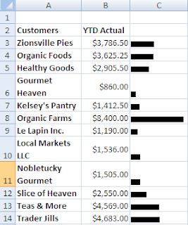
These charts are popular as they are quick and they do not take up a lot of room. You can also quickly change the font color or apply a background color to the cell to give it a little bit more polish.

Have fun with it.

USING IF and ROUND Functions to Check Balances

CHECKING TO SEE IF YOU ARE IN BALANCE
This is a handy formula to double-check your balance sheet with:


It is often easier to type in the TRUE and FALSE components first

=IF(ROUND(C4,0)=ROUND(C6,0),"in balance","out of balance")

You have to round both cell references….

Once you have done this, if you change c6 to 99.5, C10 will display In Balance.

Tip: Always test both the true and the false components. Just because one works - that doesn't mean the other does.

Breaking Worksheet Links

I hate to repeat myself but GO BUTLER!!!!!!!!!!!!!!!!!!!!!! Impressive Game. I hope that you all watching the game tonight and cheering for Butler.

It is Spring Break so this week's blog will be sporadic but I thought I would start out on the right foot and write one today.

I wanted to talk today about Breaking links between workbooks.

Now, why would you want to break your links after you went to all the trouble of setting them up? If you do have a lot of externally linked files then you know that it can take awhile to pull the files up as well as to perform calculations as more memory is required.   Breaking the links is suggested if you are going to email one or more of the files to someone or if you want to save a copy of the file for archiving or just want a static document.

It's very easy to do.

Open the workbook that has the external links

Click on the Office Button

Select Prepare

and select Edit Links to Files

In the dialog box that opens up, select Break Links.

A dialog box will warn you that this permanently converts formuals and external references to their current existing values and that this action cannot be undone.

If you don't see the Edit Links to Files selection, it means that you do not have any externally linked files. This feature does not handle links within a file - only external files.

If you break the links, it only converts externally linked formulas to numbers - any internally linked cells are unaffected.

Have a great day and watch the game tonight. It should be a good one.

Copying Pivot Tables

Saving yourself some time with pivot tables.
If you have been creating all your pivot tables from scratch each time - this trick will save you some time.

Suppose you have created a pivot table showing your Top 10 Products and you also want to create a Bottom 10.  No point in starting all over - just copy it.Look at all the time that saves plus you have the same formatting.  This is particularly useful if you are setting up a dashboard.

1. Select the pivot table
2. Copy the pivot table and place it beside the original pivot table
3. Right-click on an item (or product in this example) in the pivot table
4. Select Filter
5. Select Top 10…
6. Click the drop-down arrow beside Top and select Bottom
7. Click OK
8. Replace Top Products with Bottom 10 Products by typing over it.

How easy was that?

Have a Wonderful Easter.

Go Butler

Hey- It's 80 and absolutely gorgeous out and Spring Break is starting so I'm heading outside to enjoy the great weather while it lasts.

But let me take a minute to say GO DAWGS!!!!!!!!