Want to Learn VBA?
I've had a couple of people asking about VBA lately and wanted to tell you about a site that contacted me. They are a UK site called Best STL and they do training. They are currently offering 2 excellent Ebooks on VBA for free.
Check them out when you have a chance. I am hoping to get a CPE course on VBA out sometime next year but in the meantime you might find this information very helpful.
http://www.microsofttraining.net/vba-training-manuals.php

Software examples that you can easily understand and immediately apply to your own business needs.

Thursday, December 4, 2014
Friday, November 21, 2014
Refreshing Pivot Tables
Quick Tip for Refreshing Pivot Tables
Alt+F5 will refresh all the Pivot Tables on the sheet.
CTRL +ALT+F5 will refresh all Pivot Tables in the workbook.
Alt+F5 will refresh all the Pivot Tables on the sheet.
CTRL +ALT+F5 will refresh all Pivot Tables in the workbook.
Monday, October 13, 2014
Ebooks Now on Amazon

Just wanted to let you know that we have started putting some of our Excel Ebooks on Amazon. I have had some people who are not CPAs and who do not need CPE ask that we do that.
So, far we have 2 Excel Ebooks out there:
Comprehensive Look at VLookup and othe Lookup Functions
Excel Time Value of Money Functions
Tuesday, September 16, 2014
Setting up Ringtones for a Contact on your Iphone
Setting Up Different Ringtones on IPhone

You can set up different ringtones, text tones and even different vibrations for specific people on your Iphone. This can be very useful if you want to be able to identify certain calls but you cannot immediately access your phone.
Here are the steps.

Select the person you want to assign a specific ringtone.
Once you have their page open, click on Edit ( in the top right hand corner).
Scroll down to Ringtone; it should be set to “Default”. Click the arrow (chevron) to the right of “Default” and select a new sound.
When you select a new sound it will play it for you so that you can hear what it sounds like. If you don’t like it then try another one ringtone. That's it...
This is very useful if you have kids and you may also find it useful if you have a bothersome boss or employee :)
Thursday, September 4, 2014
Hide and Seek - Column A

Unhiding a column or a columns in a worksheet is generally pretty easy. For example, to unhide columns C and D, simply select the Column B header and drag across and select the Column E header (This in effect is selecting Column C and D) and then right-click and select Unhide.
Now, Column A however can be a different story since there is no column before it to select.
The easiest way to unhide Column A is to go to the Name box and type in A1 and press Enter.
Excel will move your cursor to cell A1
even though you can’t see it.
You can then go to Format>Cells and go to
Visibility>Hide and Unhide and then select Unhide Column.
 I ran into a situation yesterday where I could not
get this to work. However, by
selecting the entire worksheet and copying it to a new sheet all my hidden
columns displayed!
I ran into a situation yesterday where I could not
get this to work. However, by
selecting the entire worksheet and copying it to a new sheet all my hidden
columns displayed!To select an entire worksheet click on the header located under the Name Box (above row 1 and to the left of Column A)
Monday, August 25, 2014
Selecting Non- Contiguous Cells
CTRL Key

I was talking to someone the other day who had been using Excel for years but was unaware of how to select non-contiguous cells so I thought I would explain it in case you were interested. It is extremely easy.
- You select the first cell or range of cells that way you normally would.
- Then you hold down the CTRL key and select the next cell or range of cells.
- If you have another row select it (still holding down the CTRL key)
- Deselect the CTRL key when you have finished.
Yup.. that is all there is to it.
So, what can you do with this knowledge?
- Well, I love to you use this when charting.Just select the non-contiguous ranges of data you want to chart and then click Insert and select your chart type. Deselect the CTRL key.
- This is also useful if you want to format the top and bottom row of your P&L as currency. No point in selecting the top row and formatting it and then moving to the bottom row and formatting. Instead select the top row, hold down the CTRL key and select the bottom row and then apply the formatting. When finished just deselect the CTRL key.
- This also works if you have a couple of non-contiguous columns that you need to sum. Just select the first column, hold down the CTRL key and select the next column and then the next column and the next column etc. Click the AutoSum icon and all the columns will display totals.
Monday, May 19, 2014
Protect Your Workbook Structure
Protect Your Work

Anyway, in addition to protecting the cells in the sheet which I have covered in other blogs, today I want to talk about protecting your workbook's structure. It is easy to do and you will wish that you knew about this a long time ago.
These steps pertain to the entire workbook - not just a worksheet.
- Click Review.
- Select Protect Workbook which is located in the Changes grou.p

- Select Structure Option in the Protect Workbook dialog box.

- 4. Click OK.
If you select Windows, you can prevent users from changing the size or position of worksheet windows.
This tip is very useful if you are linking together several spreadsheets maintained by others.
Wednesday, February 5, 2014
TRACKING FORMULA ERRORS in SPREADSHEETS
Guest Post: J. Helstrom

Spreadsheet
formula errors may cause other calculations to also yield an error
message.
This is aggravating, especially
if you’re working with a large worksheet.
Formula errors can be fixed - the
hard part is finding all of them.
Luckily, Excel provides a handy tool for identifying formula
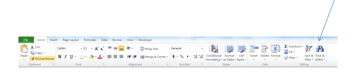
errors. It’s embedded within the Find & Select icon on the Home ribbon.
Press Find &
Select, then click on Go To Special…
or press the F5 key and then click Special....

The following dialog box appears:

Click the Formulas button and then deselect everything
except the Errors check box as shown below:

Click on OK and all errors in the worksheet are now
highlighted.
As an example, assume that a worksheet contains the
following errors:

When Find & Select…Go To Special…Formulas…Errors is
selected as shown above, the result is:

Excel has highlighted all the error messages.
If you haven't used Go To Special before - take a look at it. You can do a lot of cool things with it such as selecting visible cells only and it also allows you to find cells containing Conditional Formatting and Data Validations among other things.
Monday, January 13, 2014
JOINING VLOOKUP FUNCTIONS TOGETHER

Between the holidays, Ice Storms and dealing with my daughter's wisdom teeth removal, it has been a little while but I am still working away on my VLookup Ebook and I have to tell you I have learned some cool tricks.
This tip is a bit basic but I am willing to bet some of you have never considered it. It is a really simple idea but one that never really occurred to me until I started really looking at Vlookups.
Instead of creating two Lookup functions and then creating a 3rd column to multiply or add the numbers together – you can do it all in one.
In the example below, my Order information is in Columns C through H and the lookup table containing my data is in Columns K through R.
My lookup value is Product ID which is in Column E. I want to find the Price in Column Q and the Shipping Cost in Column R for each product and then multiply it by the quantity of product being shipped.
In other words, I want to add together the Price (Column Q) and the Shipping Costs (Column R) for each Product ID in Column E and then multiply it by the Quantity in Column G.
To do this, I clicked in cell H3, Total Price, and created a Price Vlookup to look up the Price in Column Q, typed a plus sign and then created a second Vlookup to retrieve the information in Column R. Then I put parentheses around the entire equation and multiplied it by G3 (Quantity)and then copied it down.

The
equation is: =(VLOOKUP(E3,$K$3:$R$30,7,FALSE)+VLOOKUP(E3,$K$3:$R$30,8,FALSE))*G3
Just a little faster way to do the calculation. Have fun.
Subscribe to:
Posts (Atom)

Ms. Excel- Resident Excel Geek