Protect Your Workbook Structure

Protect Your Work

If you share workbooks with others then I am sure you have experienced someone inserting or deleting a sheet and totally messing up your work. Or, that helpful person who renames the sheets for you??

Anyway, in addition to protecting the cells in the sheet which I have covered in other blogs, today I want to talk about protecting your workbook's structure. It is easy to do and you will wish that you knew about this a long time ago.
These steps pertain to the entire workbook - not just a worksheet.

• Click Review. 
• Select  Protect Workbook which is located in the Changes grou.p
• Select Structure Option in the Protect Workbook dialog box.
• 4. Click OK.

If you right-click on a sheet name after doing these steps, you will see that you can no longer delete, insert or rename a sheet. In addition, you cannot change its color or hide or unhide the sheet.

If you select Windows, you can prevent users from changing the size or position of worksheet windows.



This tip is very useful if you are linking together several spreadsheets maintained by others.

TRACKING FORMULA ERRORS in SPREADSHEETS
Guest Post: J. Helstrom

Spreadsheet formula errors may cause other calculations to also yield an error message.

This is aggravating, especially if you’re working with a large worksheet.

Formula errors can be fixed -  the hard part is finding all of them.

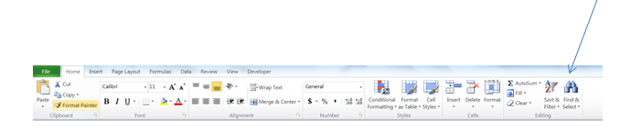
Luckily, Excel provides a handy tool for identifying formula errors.  It’s embedded within the Find & Select icon on the Home ribbon.

Press Find & Select, then click on Go To Special…

  or press the  F5 key and then click Special....

The following dialog box appears:

Click the Formulas button and then deselect everything except the Errors check box as shown below:

Click on OK and all errors in the worksheet are now highlighted.

As an example, assume that a worksheet contains the following errors:

When Find & Select…Go To Special…Formulas…Errors is selected as shown above, the result is:

Excel has highlighted all the error messages. 

If you haven't used Go To Special before - take a look at it. You can do a lot of cool things with it such as selecting visible cells only and  it also allows you to find cells containing Conditional Formatting and Data Validations among other things.

JOINING VLOOKUP FUNCTIONS TOGETHER

JOINING VLOOKUP FUNCTIONS TOGETHER


Between the holidays, Ice Storms and dealing with my daughter's wisdom teeth removal, it has been a little while but I am still working away on my VLookup Ebook and I have to tell you I have learned some cool tricks. 

This tip is a bit basic but I am willing to bet some of you have never considered it.  It is a really simple idea but one that never really occurred to me until I started really looking at Vlookups.

Instead of creating two Lookup functions and then creating a 3rd column to multiply or add the numbers together – you can do it all in one.
In the example below, my Order information is in Columns C through H and the lookup table containing my data is in Columns K through R.

My lookup value is Product ID which is in Column E. I want to find the Price in Column Q and the Shipping Cost in Column R for each product and then multiply it by the quantity of product being shipped.

In other words, I want to add together the Price (Column Q) and the Shipping Costs (Column R) for each Product ID in Column E and then multiply it by the Quantity in Column G.

To do this, I clicked in cell H3, Total Price,  and created a Price Vlookup  to look up the Price in Column Q, typed a plus sign and then created a second Vlookup to retrieve the information in Column R. Then I put parentheses around the entire equation and multiplied it by G3 (Quantity)and then copied it down.

The equation is: =(VLOOKUP(E3,$K$3:$R$30,7,FALSE)+VLOOKUP(E3,$K$3:$R$30,8,FALSE))*G3

Just a little faster way to do the calculation. Have fun.

Using Vlookup with other functions

LOOKUP FUNCTION

As I mentioned, I am writing a new Ebook on Lookup Functions and am having a blast playing around with some of these formulas.
 I started with LOOKUP. I have always wondered about it as I have always used VLOOKUP and HLOOKUP but had never seen LOOKUP used.

The Excel LOOKUP function has two forms: the Vector Form and the Array Form. Today, I am just going to talk about the vector form. This 

allows you to lookup a single value from a column. 

The lookup function is pretty straight-forward although you would never know it from its syntax.

=LOOKUP(Lookup_Value), lookup_vector, result_vector)

So, in English  this translates as:
 =LOOKUP(value you looking up, column that contains the value you are looking up, the column that contains the answer).

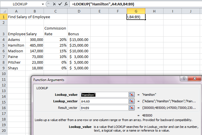
In the example below, I have an employee listing and I want to find the salary of Hamilton.  So, I am looking up Hamilton which is in Column A; that takes care of the first 2 parts of the syntax – the lookup value is A5 or “Hamilton” and the lookup_vector is Column A.
 The result or answer I am looking for is in Column B – Salary.

The equation then is =LOOKUP("Hamilton",A4:A9,B4:B9)
 

Now, this seems pretty simplistic with only 6 rows of information but you would find it useful if you had a couple of hundred or more employees. The difference between this lookup function and VLOOKUP or HLOOKUP is that there is no separate lookup table; instead, you are looking in the data itself.  

CHOOSE - A Lookup Function

CHOOSE FUNCTION

I am writing a new CPE EBook on advanced functions and starting with some of the lookup functions. I took a look at the CHOOSE function as I have always been a bit curious about it. You can do a couple of different things with it but today I am just going to talk about how to use it as a basic lookup function.

The CHOOSE function is in the lookup and reference category. The syntax is =CHOOSE(Index_number, Value1, Value2,…Value254).It returns the values from an existing list.
So- what does that mean?

Excel looks at the index number and then searches for a match in the list of values. 
It works pretty simply. =CHOOSE(3, 10,15,20,25,30) = 20.

Since the Index Number is 3, CHOOSE selects the 3^rd value in the list which is 20.

See, I told you it was simple.

Let’s go through a basic example. I have a list of employees and want to determine their tax rate based upon their filing status. For informational purposes, I have a table over in Column G and H showing the filing statuses and the corresponding tax rate. 

In the example above, I want to look up and assign a tax rate based upon the filing status shown in Column D. Instead of using a lookup table as we would with VLOOKUP, in the CHOOSE function, all the information is included in the function arguments.

The equation we would use is =CHOOSE(D4,15%,25%,28%,33%,35%).
We are telling Excel to look at D4 and then find that corresponding number in the list. Cell D4 has a filing status of 4 so Excel goes to the 4^th item in the list which is 33%  and returns it. If we copy the formula down,  Excel would show that Madison has a filing status of 3 and so would return the 3rd value in the list which 28%.

The big difference between CHOOSE and the VLOOKUP is that all the data is housed inside the function arguments rather than referencing a lookup table. If you have a lot of things you are looking for then CHOOSE could be cumbersome especially if you need to edit and update it frequently.
The advantage is that you don't need to worry about sort order, once the data is entered, or absolute cell references.