PV of Annuities using Excel

This is a guest post from Joe Helstrom, CPA and is an excerpt from his Ebook Excel Time Values of Money Function for the CPA

Present Value of Annuities


An annuity is a periodic payment of a fixed amount. The most prevalent examples are car loans and mortgages. They add the payment (Pmt) variable. The present value of an annuity deals with the value today of a future stream of fixed payments at a specific earnings rate.

Example.
Your client has just won the lottery. He must choose between $1 million paid to him immediately or $150,000 paid to him at the end of the next 10 years. He can earn 5% annually on his investments. Which option should he choose?

We have two scenarios to evaluate. The first involves $1 million today (the PV). The $1 million involves no computation. It’s already a present value. The second involves a series of periodic payments of $150,000 (Pmt) over the next 10 years (Nper) to be evaluated at an annual rate of 5%. We want to know the present value (Pv) of the annuity in the second scenario to compare to the first scenario. First, we prepare our input spreadsheet.

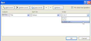
Click on the Fx button on the left side of the Formulas tab.  It will ask you to select a category.  Select “Financial”.  On the bottom, scroll down and choose PV.  Click OK.  The function arguments wizard will appear.  Complete the function arguments wizard as shown below.

Click OK. 

Once again, ignoring the sign convention, the present value of $150,000 per year over the next 10 years at a rate of 5% is $1,158,260.  Which is better – $1 million today or $1,158,260?  In this case, the better deal is to take the $150,000 per year periodic payments.

If you want to make the answer a positive number, place a minus sign in front of the payment (Pmt) input.  The answer is negative as Excel assumes that you would need to pay (cash outflow) this amount to obtain (cash inflow) $150,000 per year payments at a 5% rate.

AGGREGATE()

Excel 2010 introduced a couple of new functions. If you currently use the Subtotal() feature, you might be interested in a new function that was introduced in Excel 2010 - AGGREGATE().


The AGGREGATE() function is similar to the SUBTOTAL() function; however, it gives you greater control over what to ignore or what to include. It is particularly handy if you routinely have error messages in data that you are trying to manipulate. You can specify that you want the calculation to ignore hidden rows, subtotals, eror cells and or any combination of the the 3.

The syntax is =AGGREGATE(function_num,options, array, [k])

The function number, like Subtotal() 's , is a number that refers to the function you want to perform. Aggregate's function number has been expanded to 19.

Options allows you to specify what you want to ignore or exclude:

Array are the cells that you are trying to aggregate/subtotal.

Below is a simple example. For Java Joe's I have filtered all the data to just see customer "Cup of Joe"'s sales.

Now, I just want to add up Cup of Joe's Total Sales in Column F.

If I tried to use the SUBTOTAL() function I would get an error message since F13 has an error value.

 

Instead, I can use AGGREGATE() and tell it to ignore any error values as well as hidden rows. The answer of 1053.2 is returned.

New Keyboard Shortcut

I have been woefully behind on this blog due to family illness and upgrading CPASelfstudy.com so I apologize to people who have left me questions however I will get them all answered shortly.
CPAselfstudy.com will be down March 17and March 18 as the site is upgraded and shopping cart changed. I can't wait for this to be finished :)

Meanwhile - A quick tip.

Display Formulas with Keyboard Shortcut

This one was new to me and I have to thank Francis, the ExcelAddict, for it.
If you have a large spreadsheet with a lot of formulas, a really quick way to display them is to simply Press the Control key and the tilde button. The tilde button is the upper left of the keyboard and looks like this: ~

Press Ctrl and ~ together and your formulas will display. It works as a toggle.

If you have long formulas, you will need to widen the columns to see the formulas and then manually return them to their previous width.

Have a great St. Patrick's Day!

Excel Hero Academy - Starts Feb 1

I wanted to tell you about Daniel Ferry's Excel School. Daniel is a Microsoft Excel MVP and runs a really interesting Excel enthusiast blog. If you have not discovered it yet, definitely check it out. It’s called Excel Hero . What makes Daniel's blog interesting is that he does all sorts of things with Excel that no one has ever seen before. Some really fun things to be sure, but very important and useful business things as well.

Daniel started an Excel training course a few years back at the request of his readers It is called  Excel Hero Academy . The Excel Hero Academy has been extremely popular and is now in its third year. Registration for Excel Hero Academy (EHA3) opens on February 1.

Excel Hero  teaches you how Excel “thinks” and how to leverage that to be drastically more productive at work. This makes you a valuable commodity in today’s competitive workforce. I sat in for a week or two and was impressed with the caliber of the teaching as well as of the students.  I plan to sit in this session too now that I have some "free time".

The Excel Hero Academy is an extremely in depth, 16-week, video training program. If you can dedicate three to four hours a week for the next four months, the course will revolutionize the way you solve business problems. You will be transformed, literally, into an Excel Hero.  There is homework and I want to be clear -you need to have the time for this course - you just can't squeeze it in and think you can do it in ten minutes.   I will also state that I personally would only recommend this for high intermediate to advanced Excel users and those having an interest in learning more about VBA.


The entire course can now be accessed from iPhone and Android devices in addition to the normal web based academy access. EHA Mobile is distributed as a free app (for paid students of the academy) in both the iTunes App Store and the Android Market. And the academy forums now support Tapatalk as well.


Daniel is committed to continually improving the Excel Hero Academy and the results speak for themselves. Just take a moment to peruse the many dozens of student reviews on his LinkedIn Profile.

If you enroll in the class,  you will be glad that you did. And here is the icing on the cake. I have worked with Daniel and have secured a special $50 discount for you. To learn more and enroll in the course click here
Your $50 discount code: CPASELFSTUDY.

If you sign up let me know. I always appreciate feedback particularly when I am recommending something. Daniel and I are talking about ways to set up this course for CPE credit down the road so all comments etc are appreciated. I also want to let you know that I do receive a small commission for anyone who signs up.
Have a good week.

Custom Lists

Customizing a List
I spent a little time hunting around for Custom Lists in Excel 2010 so I thought you might be experiencing the same problem.

A custom list allows you to create a list of names or data in whatever order you want. You can then sort on this list and Excel will sort in the order that you created it in. You can also use autofill to fill in the list.
People typically use it to create lists such as  product lines or sales regions.  You can sort products or sales regions in alphabetical order but perhaps you want to sort by highest revenue generator? - that is where the custom list comes in.



Click on the File tab
Click on Option
Click on Advanced on the left side of the dialog box
Scroll down until you see Edit>Custom Lists

Make sure that your cursor is on New List  and then click in the right column entitled "List Entries" and type a name and then press Enter. Continue until all the names are entered. In the example to the below I typed different sales regions in the order I want them to sort.

Once you complete the list, click Add and it adds it to Microsoft's existing custom list of days and months.

If you already have a list, you can simply import it instead of typing them in.


Click OK.

Go to an Excel worksheet and type in the word West and then use the autofill handle to copy it down and you will see that West, Mid Atlantic, New England etc display in the order specified in the custom list.
If you go to the Data tab and click Sort and  click on Custom List.. under Order you will see the sort list there also.

Click OK and the Custom Lists dialog box opens.