Document Inspector

Our CPE Course, Spreadsheet Controls Under Sarbanes-Oxley 404, is being piloted and hopefully will be for sale by the end of the month on our website cpaselfstudy.com . While writing the course, we took a look at what Excel features would be helpful for setting up controls and I wanted to tell you about the Inspect Document feature.

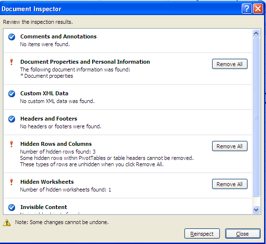
This is a new feature in Excel 2007 and what it does it is "inspect" your worksheet and tell you if you have hidden worksheets, personal information, comments, tracking changes etc.

So, from an audit and/or control perspective, this might be something you want to look at when reviewing a spreadsheet. From an end user's perspective, you might want to check this before distributing a workbook to make sure that there is nothing in the workbook that you don't want others to see.
It is very easy to use.

• Click on the Microsoft Office button
• Select Prepare.
• Click Inspect.

Excel inspect the worksheet and returns with its findings. In this case, it found 3 hidden rows and 1 hidden worksheet.

You then have the option of removing what Excel has found.

Disappointingly,the Inspect Document feature did not find  my invisible cell, (I changed the cell font color to white, so that the cell was invisible being white font on white background.); however, I think you will still find it useful.

The Document Inspector is also in Word and PowerPoint.

Converting Text with a trailing CR to a Number

,Don't you just hate it when you import data and see the dreaded CR at the end of a number. You know that Excel automatically treats any cell content as text if it is a mix of numbers and text. This of course is a huge problem if you need to actually use that cell value in a calculation.  Below is a way to convert the content by using the LEN function and the LEFT function.

• The LEN sounds like a useless function but it actually very powerful - it counts the number of characters in a cell =LEN(text). 
• LEFT is a text function and it extracts the specified number of characters =LEFT(text, number of characters).

The LEN function counts the number of characters in the cell and the LEFT function tells Excel to extract everything except for the last 2 characters in that cell. I then multiplied it by -1 to make it negative.

So, in the example above, if you break it down, Excel looks at the LEN (A20)-2 and evaluates that as 5-2 which of course is 3 so now it would read =LEFT(A20,3)*-1. Excel would treat that as =100*-1 and the resulting answer would be -100.



A lazy way to get rid of error messages

People spend a lot of time using IF statements and/or  IFERROR so that error messages do not show up in a spreadsheet but if you are in a hurry and need to present your data- here is a lazy way to fix it so that they don't display in a printed report.
Simply go to Page Setup and click on the drop-down beside Cell Errors as: and select

Changing a Cell from Text to Number

If you have imported data from different general ledger programs you might have run into the frustration of  finding that your numbers were imported into Excel as text.  An easy way to turn your text back into a number so that you can perform a mathematical function with it is to right-click on it and select Convert to Number.

Another alternative is to use Text to Columns.

First, select the cell containing the value and then select Text to Columns under the Data tab and at Step 3 select Date and then Finish.

Surprisingly, this will convert text back into a number.

Match Function

I'm putting some stuff together for a presentation I am doing for the Institute of Internal Auditor's Indianapolis chapter in November and thought I would talk about the MATCH Function. The MATCH function can be very useful if you want to compare to lists.
In the example below, I have a current inventory list and an obsolete inventory list. I want to compare the 2 lists and make sure that there are no obsolete parts on the current inventory list.

In Column A I have the current part numbers and in column D I have a listing of obsolete parts.
In column G, I want to double-check to make sure that an obsolete part is not on the current list in Column A. So, I select G2 through G6 as this is going to be an array formula and type =MATCH(A2:A6,D2:D6,0) and then I press Control +Shift+ Enter, also called CSE. G2 through G6 are populated either with N/A messages or as you can see in G3 a number.   The number 4 in G3 is telling us that A3 has a match and that it is the 4th value in the other list.
 If you look down the obsolete part list, you can see that the 4th value of XYZ-124 is the same as in the second row of the new inventory list.  Now, this gets the work done but it doesn't really look that great with all the N/As and if you had a long list it would be hard to differentiate the error messages from the numbers.

We can make this more elegant by putting the MATCH function inside of IFERROR, a new Excel 2007 function.  In the example below, I selected G2.G5 again and typed =IFERROR(MATCH(A2:A6,D2:D6,0)," ") and then pressed CSE. All the error messages now display as a blank so it is much easier to see the match.