JOINING VLOOKUP FUNCTIONS TOGETHER

JOINING VLOOKUP FUNCTIONS TOGETHER


Between the holidays, Ice Storms and dealing with my daughter's wisdom teeth removal, it has been a little while but I am still working away on my VLookup Ebook and I have to tell you I have learned some cool tricks. 

This tip is a bit basic but I am willing to bet some of you have never considered it.  It is a really simple idea but one that never really occurred to me until I started really looking at Vlookups.

Instead of creating two Lookup functions and then creating a 3rd column to multiply or add the numbers together – you can do it all in one.
In the example below, my Order information is in Columns C through H and the lookup table containing my data is in Columns K through R.

My lookup value is Product ID which is in Column E. I want to find the Price in Column Q and the Shipping Cost in Column R for each product and then multiply it by the quantity of product being shipped.

In other words, I want to add together the Price (Column Q) and the Shipping Costs (Column R) for each Product ID in Column E and then multiply it by the Quantity in Column G.

To do this, I clicked in cell H3, Total Price,  and created a Price Vlookup  to look up the Price in Column Q, typed a plus sign and then created a second Vlookup to retrieve the information in Column R. Then I put parentheses around the entire equation and multiplied it by G3 (Quantity)and then copied it down.

The equation is: =(VLOOKUP(E3,$K$3:$R$30,7,FALSE)+VLOOKUP(E3,$K$3:$R$30,8,FALSE))*G3

Just a little faster way to do the calculation. Have fun.

Using Vlookup with other functions

LOOKUP FUNCTION

As I mentioned, I am writing a new Ebook on Lookup Functions and am having a blast playing around with some of these formulas.
 I started with LOOKUP. I have always wondered about it as I have always used VLOOKUP and HLOOKUP but had never seen LOOKUP used.

The Excel LOOKUP function has two forms: the Vector Form and the Array Form. Today, I am just going to talk about the vector form. This 

allows you to lookup a single value from a column. 

The lookup function is pretty straight-forward although you would never know it from its syntax.

=LOOKUP(Lookup_Value), lookup_vector, result_vector)

So, in English  this translates as:
 =LOOKUP(value you looking up, column that contains the value you are looking up, the column that contains the answer).

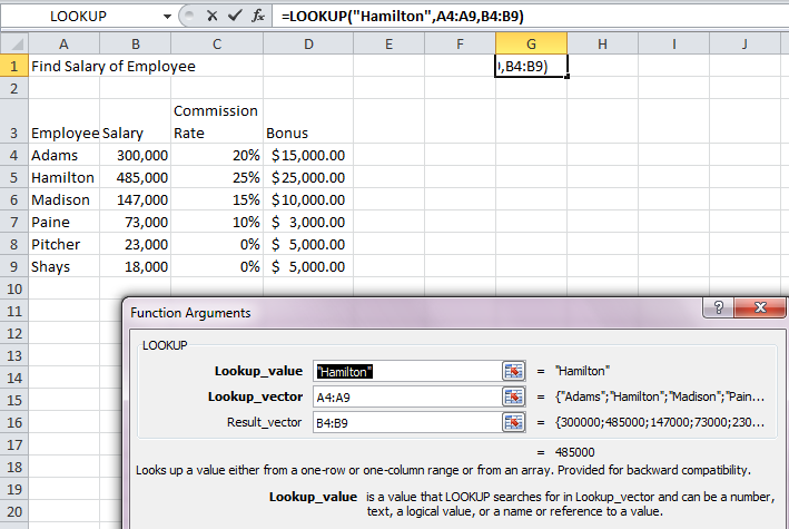
In the example below, I have an employee listing and I want to find the salary of Hamilton.  So, I am looking up Hamilton which is in Column A; that takes care of the first 2 parts of the syntax – the lookup value is A5 or “Hamilton” and the lookup_vector is Column A.
 The result or answer I am looking for is in Column B – Salary.

The equation then is =LOOKUP("Hamilton",A4:A9,B4:B9)
 

Now, this seems pretty simplistic with only 6 rows of information but you would find it useful if you had a couple of hundred or more employees. The difference between this lookup function and VLOOKUP or HLOOKUP is that there is no separate lookup table; instead, you are looking in the data itself.  

CHOOSE - A Lookup Function

CHOOSE FUNCTION

I am writing a new CPE EBook on advanced functions and starting with some of the lookup functions. I took a look at the CHOOSE function as I have always been a bit curious about it. You can do a couple of different things with it but today I am just going to talk about how to use it as a basic lookup function.

The CHOOSE function is in the lookup and reference category. The syntax is =CHOOSE(Index_number, Value1, Value2,…Value254).It returns the values from an existing list.
So- what does that mean?

Excel looks at the index number and then searches for a match in the list of values. 
It works pretty simply. =CHOOSE(3, 10,15,20,25,30) = 20.

Since the Index Number is 3, CHOOSE selects the 3^rd value in the list which is 20.

See, I told you it was simple.

Let’s go through a basic example. I have a list of employees and want to determine their tax rate based upon their filing status. For informational purposes, I have a table over in Column G and H showing the filing statuses and the corresponding tax rate. 

In the example above, I want to look up and assign a tax rate based upon the filing status shown in Column D. Instead of using a lookup table as we would with VLOOKUP, in the CHOOSE function, all the information is included in the function arguments.

The equation we would use is =CHOOSE(D4,15%,25%,28%,33%,35%).
We are telling Excel to look at D4 and then find that corresponding number in the list. Cell D4 has a filing status of 4 so Excel goes to the 4^th item in the list which is 33%  and returns it. If we copy the formula down,  Excel would show that Madison has a filing status of 3 and so would return the 3rd value in the list which 28%.

The big difference between CHOOSE and the VLOOKUP is that all the data is housed inside the function arguments rather than referencing a lookup table. If you have a lot of things you are looking for then CHOOSE could be cumbersome especially if you need to edit and update it frequently.
The advantage is that you don't need to worry about sort order, once the data is entered, or absolute cell references.

Alt plus = to quickly sum

I just picked up a quick way to quickly total a large set of numbers in Excel 2007/2010 and I wanted to share it with you.   With this tip you select the data and then press the Alt Key and then the equal sign key.

Below is a simple table of data.
Simply select from A3 to F9 and then press the Alt key and the Equal sign.
Alt+=
This will automatically total Column F and Row 9.

It is pretty flexible - I  get the same result if I select A4 to F9 or B4 to F9.
Have a great weekend.

If  you are looking for more great tips check out my Tools and Tips CPE course for Accountants.
http://www.cpaselfstudy.com/item_115/Excel-Tools-Tips-for-the-Accountant.htm

SUMIFS

Excel  2007 and Excel /2010 offers some new functions that go beyond the simple SumIf and CountIF as they allow you to test up to 127 conditions. The new functions are Sumifs, CountIfs and AverageIfs. (Excel 2003 does not offer AverageIf but Excel 2007 does). They are called the Plurals due to the S at the end of the function.

They all work the same way and the syntax is similar. We are going to add up the Sales for Pam's Tea Parlor if the Country of Origin is China  and the Quantity purchased is greater than or equal to 3.   Only 2 rows meet all the criteria and I have highlighted them in purple so they were easy for you  to find.

Here is the formula: =SUMIFS(G7:G21,A7:A21,A7,C7:C21,"China",F7:F21,">=3")

Let's walk through the steps:
SYNTAX
SUMIFS(sum_range, criteria_range1, criteria1, [criteria_range2, criteria2], ...)

Sum_range
The sum range is G7.G21
This is the range of cells that you want to do the math on. In our case we want to sum up the Sales column.

Criteria_range1 is A7.A21
This is  first range is the criteria that everything else is based off of. In our example, we are filtering our data  based upon  Column A where the customers are.

Criteria1  is "Pam's Tea Parlor" or A7. 
This is the criteria that Excel is going to look for in the Criteria_Range1 which in our case is Column A.
I used A7 instead of typing "Pam's Tea Parlor" since it saves me worrying about typos and I was not copying this formula so I didn't need to worry about relative and absolute cell references. If you do type in text then you need quotation marks.

So far, we have told Excel to sum the sales if the Customer is Pam's Tea Parlor.
The criteria1  selection  must match something in Criteria_range1  and the criteria2 selection must match something in the Criteria_range2 selection etc.  All further conditions step off Criteria1.

The remaining sytnax is optional and you can continue adding up to 127 criteria. We are only going to add two more- Origin of China and Quantity greater than or equal to 3.

Criteria_range2 is C7.C21
We area filtering our data further and limiting our interest to teas from specific locations that have been ordered by Pam's Tea Parlor

Criteria2 is "China"
Criteria2 must match an item in the column that was specified in Criteria_range 2. We are only looking for teas from China that were ordered by Pam's Tea Parlor. Again, text needs to be in quotations.

Criteria_range3 is F7.F21
This is telling Excel that our next interest is Column F - Quantity

Criteria3 is >=3
Quantity greater than or equal to 3. If you do not put quotations around >=3, Excel will generally add them in even though it seems incorrect. The syntax on SUMIF and SUMIFS is not the same as an IF function.

However please be aware that I could only test for one criteria per column unless you can use a wild card to meet your criteria.

In other words,  I can only test for one country of origin unless I can use a wild card. Excel would not provide an answer if  I had wanted to sum sales for Pam's Tea Shop if the tea came from China and Korea and the quantity was greater than or equal to 3.  I could only select a single country of origin.