This is a guest post from Joseph Helstrom, CPA.

Adding VLookup as a Control for Your Month-End Workpapers

When closing for the month, many use an Excel workbook to reconcile balances to the general ledger.  As the general ledger changes, do you have a process in place to easily determine that balances previously reconciled still tie to the general ledger?  If not, using Vlookup on each reconciliation worksheet provides a quick and easy way to accomplish this control.

Usually, the month-end balance from a reconciliation worksheet is at the bottom of the worksheet.  Below this balance, you can enter the associated general ledger account number to be used in a Vlookup formula.  After the account number and Vlookup formula have been entered in each workbook, all you need to do is cut and paste the most recent general ledger balances into a separate worksheet.  The Vlookup will display the most recent balance and you can use conditional formatting to highlight whether the two balances are within a tolerable error limit.

The example below assumes that the AR Trial Balance has been created and the total needs to be compared to the general ledger.  There is a worksheet labeled “Accounts Receivable” and a separate worksheet labeled “General ledger”.

The general ledger account for accounts receivable has been entered at the bottom of the Accounts Receivable worksheet and a Vlookup formula is used to compare this total to the amount in the General Ledger worksheet.

The Vlookup function is searching for a worksheet titled “General ledger” in the same workbook.  The key to making this work is that you never delete this worksheet.  When the general ledger changes, simply paste the new general ledger data over the old data in the same worksheet.

For Vlookup to work, the lookup value, in this case the general ledger account number, must be in the leftmost column of the General Ledger worksheet (In this example, column A).  The general ledger data is in columns A and B and the account balance is in column 2 (which is the B column).  The FALSE range lookup value is used to indicate an exact match.  The example general ledger is shown below.

Why use the entire columns of A and B?  That way, if general ledger accounts are added, we’re not constrained by a limited range.  This is important as we want to paste over this data again and again without using new Vlookup formulas each time. 

To calculate any differences, subtract the general ledger balance from the reconciliation balance.  Use the ABS function in the formula since we just want to know the absolute amount of a difference and do not need to know whether it is positive or negative (ABS provides the absolute value of a number).   More.....https://cpaselfstudy.com/vlookup-control/

TextJoin - An Excel 2016 Text Function

If you need to join a lot of text together in a string, check out TEXTJOIN.

It is a text function that was introduced in Excel 2016 to join text in cells together.
Initially, you might think that the function is not worth investigating. After all, we already have the ampersand (& ) as well as the CONCATENATE function to join text together.
However, TEXTJOIN has a decided advantage if you need to join multiple cells together because it only requires you to specify the delimiter once.
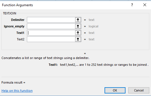
The syntax is =TEXTJOIN(delimiter, ignore empty, text…)

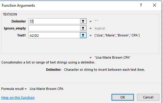
Let me give you a simple example using a person’s first, middle and last name and their professional designation.

If we used CONCATENATE, the equation would be : =CONCATENATE(A2,” “,B2,” “,C2,” “,D2). With TEXTJOIN the equation is  =TEXTJOIN(” “,,A2:D2).

and this result would display: 

Lisa Marie Brown CPA

Clearly, TEXTJOIN is a bit simpler and a bit more elegant if you have a lot of cells that you want to join together and you want to use the same delimiter throughout.

Different Delimiters
You can use different delimiters if you wish and it is still simpler than CONCATENATE as well.
In this example, I wanted spaces after each of the names but I wanted a comma before the professional designation so I used =TEXTJOIN(” “,,A2,B2,C2,”,”,D2) and Excel displayed  the following result.

Lisa Marie Brown , CPA

So, add TEXTJOIN to your arsenal of text functions if you have Excel 2016.

Searching for Files with Keywords

Using Keywords to Find Your Excel Files

If you have lots and lots of files, you know how difficult it can be to locate one, particularly if you did not name it well. Plus, let's face it, memories don't improve with age.

So, here is a solution. When you create the file, add some keywords, a title and the author's name to make it easier to locate the file at a later date.

It is very easy to do, however, you do have to remember to add this information so that you can search for it later:)

1. Click on File and then select Info.
2. Click the Properties drop-down arrow - located over on the far right side of the screen and then select Advanced Properties.
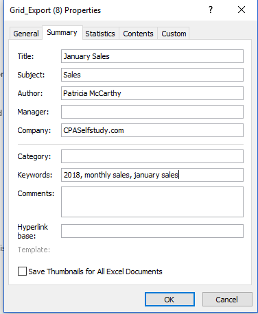
3. Click on the Summary Tab and enter keywords that relate to the file. 
4.  Click OK.

 To search, simply go to the Windows Explorer window and in the search box, located on the far right of the window, type in one of your keywords.  Your file should display. You can also search on author, a category or a title as well.

Lots of options to find your file.