Viewing the Supporting Detail behind the Pivot Table

Pivot tables are used to summarize large volumes of data however sometimes you want to see the underlying information that supports a number in the pivot table.

  The good news is that it is very easy to do - all you have to do is double-click!

Below is an example to illustrate:
I have a pivot table that is showing shipments by customers and their total order amount.

I want to see the supporting data for my customer Backpedal Cycle Shop at row 13.


When I double-click A13, the Show Detail dialog box pops up.
This dialog box allows me to specify what supporting detail I want to see.

 I selected Product Name and clicked OK.

Excel then displays the detail for Backpedal Cycle Shop's orders by Product Name.

In Excel 2010, it actually displays the supporting detail in the pivot table itself. In earlier versions, it places it on a new sheet. Notice all the detail is indented to make it easier to see.

A minus sign now appears to the left of Backpedal Cycle Shop. If you click the minus sign the detail will disappear and a plus will be display. Click again and the detail appears.

More on Slicers- Formatting & Connecting

More on Slicers - Formatting and Connections..

You can also do a bit of formatting with your slicers.
Click on a slicer that you have created and you will see a new contextual ribbon called Slicer Tools.

From here, you can change the size of a slicer as well as apply a formatting style.
If you look at the far left of the ribbon, you can see Slicer Caption which allows you to change the display name of the slicer.
If you select Slicer Settings you get the following dialog box.

The Slicer Settings dialog box also allows you to change the name of the field or the caption but it also allows you to determine different sorting and filtering parameters.




The other very interesting item on this ribbon is the Pivot Table Connections icon (2nd button on the ribbon). I have not played around a lot with this feature yet but what it allows you to do is share a slicer among different pivot tables. In other words, if you have 3 different pivot tables using the same data, you only need to set the slicer once and connect it so that the one slicer controls all 3 of the pivot tables. 

 This looks to be a pretty cool feature and should be particularly useful when doing presentations. Have fun playing around with it. I know I plan to.

Slicers! A better way to filter Pivot Tables (Excel 2010)

If you use pivot tables, then you already know they are one of the best features in Excel. The good news is that Excel 2010 actually makes using pivot tables even better with their creation of the slicer. Sounds like a Ron Popeil commericial doesn't it?  It slices, it dices.....................

Anyway, in earlier versions of Excel, you could filter pivot tables but the field you filtering had to be in the pivot table and the drop-down box would just display the text "multiple fields" so no one at a glance knew what the heck you were filtering and displaying in your pivot table.

The slicers are essentially dialog boxes containing all the field names that remain on the screen. You select the ones you want and the data in the pivot table adjusts to what is specified.

Here are the steps

• Click in your pivot table

• Click on the contextual Options tab
• Select Insert>Slicer
• Click Insert Slicer...

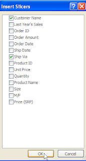
A dialog box of all the field names that comprise your data (not just the data in the current pivot table) displays

• Select your field (s)
• In this example, I selected multiple fields -Ship Via and Customer Name

• Click OK

The selected slicers display on the spreadsheet

• Click on the fields that you want to see.

 To select multiple fields in Ship Via for instance, select the first one and then hold down the control key to select the next.     

In my example, I selected Fed Ex, Parcel Post and UPS from the  Ship Via slicer and I selected the Backyard Cycle Shop as the customer I was interested in.

The pivot table now displays only data  for that one customer if one of those 3 specified carriers were used.

How cool is that.  The slicers stay there on the page and can be moved around so now you can clearly see that is being filtered and displayed in the pivot table. Think how useful this could be on a dashboard.                                                                 





Pivot Table - Rolling Up Dates

I am in the process of updating my Pivot Table course for Excel 2010 so I thought I would go through some of the fun things you can do with pivot tables here in my blog.  The new slicer function is extremely cool but let me start with a few basics before I get there. Today, I want to talk about rolling up dates in a pivot table.

You can do it in all the versions - it is just a little bit easier in Excel 2010.

• First, you click in your data and select Insert>Pivot Table
• Then drag the field from the Field List Dialog box to the specified area.
• In my case I dragged Order Date to the ROW, Ship Via to the COLUMN and Order Amount to the VALUES section

to create the pivot table below.

 

 

There are a  lot of orders here so the pivot table is not that useful. It would be useful if I could see orders by month, quarter or by year. In other words, I want to "roll" up the dates and view it by month and by year.

• You can either right-click on the dates

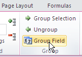
• or in Excel 2010 you can also click on the Group Field icon on the contextual Pivot Table toolbar.

Either of these methods brings up a Grouping date dialog box.

At the top, it displays the newest and the oldest data.

•  In this dialog box, I selected months and then held down the Control key to also select Years.

(It is recommended that you always select years - if you do not and there is more than one year of data, Excel will not differentiate and will instead treat it all as a single year).

Now, the orders in my pivot table display by Year and by month and is much more useful than the first pivot table.








You can hide the individual months by clicking on the button immediately to the left tof the year or by right-clicking and selecting Expand/Collapse.

Also, if you take a look at the pivot table field list, you will see that you have a new field called Years that did not exist before. You can move this field around in the pivot table and you can even use it in a new pivot table that is based upon this one.