Frequency Distribution

I hope you all are enjoying this great weather. I've been working away preparing for a couple of seminars that I am doing in May and I have to tell you I've been having a blast learning all kinds of new tricks and tips that I will be sharing shortly with you. 

Today, I thought I would talk about the Frequency functions. This was quite useful to me when I taught at Butler. For all you of you instead of grades- consider using it to track warranty information or perhaps returns or HR data such as salary levels in your organization. If you think about it, I am sure you will find a couple of uses for this.

Frequency Distributions


A frequency distribution allows you to measure performance of one item against others. A good example would be a comparison of students in a class and the grade category that they fall into. Again, consider tracking returns of an item by color or even item number. Other possibililies include a breakdown of prices for a product line or even ages or education of your workforce.
A frequency distribution is a table where data in a spreadsheet is counted into bins. It is a good habit  double check your calculation - to verify that the number of items in your input range equals the number of observations in your answer. Use a COUNT function on the input range and the sum function on your answer.

To create a frequency distribution

1. Create a set of numbers to use as bins. Keeping with our grading metaphor, you may want to have five (5) bins such as the following: 100, 89, 79, 69 and 59.

In our case, we are asking Excel to group grades so that we can see the number who earned a grade between 100 and 90 as one category (the A group), those who earned a grade between 80 and 89 (the B group) etc. all the way to a count of those who earned a grade between 0 and 59.

The bins created are in Column F. The description was added in Column D and E is solely for clarification and documentation and is not used in the calculation.

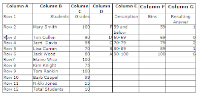
2. Select the cells where you want your answer to go. In this case, select G2.G6.

3. Type = Frequency (and then select the input range. In this case you would select C2.C11.

4. Type in a comma and then select your bin range. In this case F2.F6.

5. Type a closing parenthesis. Your formula should look like =frequency (c2.c11, f2.f6)

6. Now the important part - press CTRL+SHIFT+ENTER. The resulting frequency distribution should appear and resemble Column G. The resulting formula should look like {=frequency (c2.c11, f2.f6)}

So, what does this tell you? It tells you that in the A bin which are grades between 90 to 100 (inclusive), 6 people fell into that category whereas only 2 people ended up in the C category which was from 70 to 79 inclusive.
A couple of comments:
Excel puts the brackets around the formula to show that it is an array. If at step 2, you only selected G2 and after going through the other steps, you copied the formula down- the answer would be wrong, Because this is essentially an array formula, you need to select all the cells G2.G6 at one time for this to work.

Also, bins must be numeric. In the example below, I want to figure out how many people have less than a high school education but my data and the bins must be numeric. Again, the description is purely for the user- it is not used in the calculation. As mentioned above, it is a good idea to sum your Frequency and then count your observations to make sure that the number are the same.  In the example below, my frequencies total 40. If I counted the number of people in my data, it should total 40 people otherwise there is a problem somewhere.

Scenario Manager - What-IF Analysis

Scenario Manager - What IF

Where has the week gone? It is Wednesday already! I received some excellent news yesterday. After five and half months, CFO Resources / CPASelfstudy.com has finally been approved as a CPE sponsor in New York. Hurray!

But I do need to finish up my What-IF section by talking about Scenario Manager. This is a cool feature and is available in all versions of Excel- you just have to figure out where Microsoft hid it. In earlier versions, you have to go to Tools>Addins. In Excel 2007, look under the What-if icon on the Data ribbon.


Scenarios allows you to substitute values in a number of cells and save that condition under a unique name. By invoking different scenarios, up to 32, you can easily demonstrate to your customers and managers the impact of different events or possibilities.

• A scenario is particularly useful in creating budgets and forecasts when you have a few key variables that are subject to change.
• You can use scenarios to forecast different outcome based upon changes to these variables in your model. You can create and save these scenarios with different names and then display them.
• To compare several scenarios, you can even create a report that summarizes them on the same page- similar to a data table. The report can list the scenarios side by side or summarize them in a pivot table.
  
  Before creating a scenario you need to determine which cells will be changed. Normally these should be your input or changing cells. You can have up to 32 changing cells in a scenario.

To Use Scenarios
1. Click the Data tab on the Ribbon.
2. Click the What-if Analysis button and click Scenario Manager from the menu.
3. Click the Add button.
4. Enter a name for your scenario in the Scenario Name box.
5. Click in the Changing Cells box.
6. Hold down the Ctrl key and select the cells in your worksheet that you wish to change.
7. In the Scenario Values dialog box, enter new values.
8. Click OK.
9. To Apply a Scenario to your worksheet, select the desired Scenario and then click Show.
10. Click Close.

Careful! Adding scenarios to a workbook will change the underlying data so it is highly recommended that you save a backup of your original workbook first.
Once you have created your scenarios, you can create side-by-side Summary reports to compare your scenarios.
Take a look at it if you get a chance. Tomorrow I will try to post some screenshots and an example.

Spinners - What IF

Spinners

I forgot to mention that down at the bottom of the blog, is a link to a video I did on Goalseek. Check it out when you get a chance. And don't forget to feed my little fishies....

Today, I wanted to talk about spinners. If I have time I will put some screen shots out on the different spinner steps but as usual I am behind schedule :)

A spinner, or Excel refers to it as a scroll bar sometimes, allows you to click and select different numbers. A spinner allows you to generate a large number of scenarios that vary each input between its high and low value. A spinner is a button that is linked to a given cell. As you click the spinner button the value of the linked cell changes and you can see the impact of these changes. This can be really useful if someone else is going to use the worksheet and is not very knowledgeable about Excel.

To create a spinner:
If the Developer tab is not available, display it by clicking on the Microsoft Office Button , and then click Excel Options. In the Popular category, under Top options for working with Excel, select the Show Developer tab in the Ribbon check box, and then click OK.

++If you are using Excel 2003, you would find the spinner button on the Form Toolbar. You can find the Form toolbar under the View menu.

1. On the Developer tab, in the Controls group, click Insert.
2.Under Form Controls, click Scroll bar .
3. Click the worksheet location where you want the upper-left corner of the scroll bar to appear.
4. Right-click and select Format Control
5. Select the values you want
6. Click OK
++ Please note that the maximum value cannot exceed 30000

For spinner control set the cell link to an adjacent cell on the form.
If the cell is locked, the spinner control will generate a warning when you use it after protecting the worksheet. Avoiding this problem is easy—with the worksheet unprotected, simply right-click on the cell associated with the spinner and choose Format Cells... Select the Protection tab and deselect the Locked checkbox. You can then protect the worksheet and use the spinner control without any problems.

Goal Seek - What If with Excel

Okay- my theme this week, in case you have not guessed, is What-If. Let's talk about Goal Seek. This is one feature that some people are familiar with simply because you were able actually find it in early versions of Excel under the Data menu unlike Solver and Scenario Manager that are add-in programs that you actually have to look for.

Goal seek is great to use if you are doing a simple and quick what-if. The reason for this is that Excel only allows you to change one cell with Goal Seek as opposed to 32 in Scenarios! Also, the cell you are changing cannot contain a formula. However even though it is a bit limited, it is still useful to know how to use it when you have something simple to determine. It certainly beats typing in a number, pressing Enter and looking at the answer and then typing in another number and seeing what that answer is... yes... some people still do that.. you know who you are. Try Goal Seek instead.

Goal Seek

Goal seek allows the user to find a specific value for a cell included in a calculation by changing one other variable in the equation. It is a wonderful tool if you are trying to work through a what-if scenario.
For example, suppose you want to obtain a home loan but can only afford $800 a month. With Goal Seek, you could determine the maximum home purchase price that you could afford quickly.

Goal Seek requires 3 parameters.
1. The cell you want to change. In the example above, this would be the loan amount.
2. The value to which you want to change the target cell.
3. The cell you want to change to achieve the target amount.

To Use Goal Seek
1. Click the Data tab on the Ribbon.
2. Click the What-if Analysis button and click Goal Seek from the menu.
3. In the Set Cell Box, type the cell reference of the cell that contains the formula you want to change.
4. In the To Value box, type in the value to which you want to change the cell.
5. In the By changing cell box, enter the cell reference of the cell that contains the value you want to adjust.
6. Click OK.
7. Click OK.

I have a screenshot below example below: I wanted to change the current monthly payment in H6 to $800 by changing D6 which was the value of the loan.

2 Input Data Table

Two Input Data Tables

It's Monday already and what a gorgeous fall day it is too - only problem is that it is still August! Autumn is my favorite season but I think it is a bit too early this year. I had a great weekend - spent quite a bit of it shopping which is always fun although I got to spend a fair amount of time outdoors. I even made it to the movies with my daughter to see Bandslam.

Anyway, last week I talked about 1 input data tables and told you that I would talk about 2 input data tables this week. The example I am using is a loan example since this is the most common use but tomorrow I'll give you some ideas of what else you can do with this.
Data Table- Two Inputs
In the example below, we are testing the effects of different interest rates and the investment amount so we are using both a row and a column input.

The row input is years and the column input is the interest rate. An input cell is one in which each input value from a data table is substituted.

Click in cell D6 and type: =B14.
Select the cell range D6:H12
Click the Data tab on the Ribbon.
Click the What-if Analysis button on the Data Ribbon and click Data Table from the menu.
Click in the Row Input Box and type: B10
Click in the Column Input Box and type: B8 as shown
Click OK

and Voila- you get the following:

Give it a shot and see what you think.

Data Tables - What-If Analysis

Okay- I couldn't sleep so I figured I would get a jump on the day's work and get my blog finished up early. As I mentioned before I am working on an Advanced Excel Analysis Tools Ebook for a course I am teaching at the Indiana CPA Society in September. One of my associates was fascinated with some of the Excel What-IF features I am covering so I thought I would share part of that with you. Today or tonight I guess- I am going to talk about one variable data tables.

DATA TABLES
A data table allows you to study the effects a range of values has on a formula. This is a timesaver as you only need to set the formula up once. A one-variable data table is a range of cells that shows the results of substituting different values in one or more formulas. Data tables are actually array formulas which allows them to perform multiple calculations at once. In other words, you can see a number of different scenarios at a single glance.
There are one-input and two-input tables. We are just going to cover one-input tables today.

ONE INPUT DATA TABLES
Input values can be either listed down a column or across a row. Formulas used in the data table must refer to the input cell which is the cell in which each input value in the data table will be substituted. Any cell can be the input cell.
Type the list of values you want to substitute in the input cell either down one column or across one row.


To Create A One-Input Data Tables (General Steps for Excel 2007)
1. Type the list of values you want to substitute in the input cell either down one column or across one row.
2. Enter the formula you want to use. If the data table is in column format, enter the formula in the first blank cell above and to the right of the top of the table. If the data table is in row format, type the formula in a blank cell to the left of the first value and one cell below the row that contains the values.
3. Select the data table, including the formula.
4. Click the Data Ribbon.
5. Click the What-if Analysis button on the Data Tools group and select Data Table from the menu.
6. Enter the input cell (the value that you want to substitute with the values from your data table). If the data table is in a column, enter the cell reference in the Column Input text box. If the data table is in a row, enter the cell reference in the Row Input text box.
7. Click OK.

Clear as mud? Okay - let's go through a specific example.

We are going to create a one variable data table. The variable that is going to change is the interest rate. This is also considered the input cell. The Data Table Calculation will look at the PMT formulas, the input cell (interest rate) and the cell we want to change (payment amount).

Basically, we have a column of interest rates and we want to determine what the monthly payment will be at each different rate.


(Click on the picture for a larger view. Sorry, I need to figure out how to add files out here). Email me if you want the file.

• Observe the cell range D6.D12 which contains the interst rates. (highlighted in green).We have created a data table that we are going to use for substitute down payment values. We want to see how different rates will affect the monthly payment value.
• In cell E6 type: =B14 and press Enter. [B14 is the PMT calculation]
• The formula in cell E6 is the one whose values we want to display which in this case is the Payment Amt.
• Select the cell range D6:E12 and click the Data Ribbon.
• Click the What-if Analysis button and select Data Table.
• Click in the Column Input Box and type: B8
• Click OK
  Below is data table showing our results based upon the down payment values in our data table and our interest rates.
  
  
  
  

Look at all the different payments or scenarios if you will that you can see at once. Tomorrow or is it Thursday, I will show you an example of a 2 input variable. In that example, we will have interest rates and years as the 2 variables that change. Hey- this should be very handy if you are thinking of buying a new car or a new house however if you think about it, you can apply this to a lot of business situations. I'll give you an example tomorrow but see what you can come up with on your own.

Patricia