Season's Greetings!

Merry Christmas and a Happy New Year.
Best wishes to all of you for the coming year.

I'll be back blogging after the New Year.

Patricia

When your X axis are numbers

You get to be my guineau pigs. I played around and created some Excel videos about a year ago and put a few on YouTube and then I just never got back to it.  However, I am finishing up a self-study CPE course on Excel Charting and thought that perhaps creating a selfstudy video course would be a nice course since charting is so visual. So, anyway, this is my first crack at it. 

In the video, I talk about the problems of charting when your X axis are numbers instead of text. As you can see from the screenshot below, the chart has a few problems and does not display the selected data in Column A and B very well. To see how to solve the problem, click on the video.

When you play the video, click the icon on the far right to get it to full screen mode.

Let me know what you think. If you can't access the video here, check it out on YouTube.

Extracting Text of Different Lengths

Use the Search function to separate text

Most people are familiar with LEFT, RIGHT and MID as ways to separate text and they are useful -
but only when all the cells have the same number of characters.

If you want to separate employees' names or emails you can't use LEFT, RIGHT and MID by themselves because all the names and emails are different lengths. This is where the SEARCH command comes in.

In the example below, I want to separate my first name from my last name so to do that I need to combine the LEFT function and the Search function.

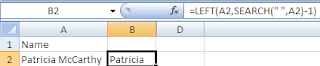
The actual function is =LEFT(A2,Search(" ",A2)-1.

Excel searches A2 for a space as denoted by the empty quotation marks, in the formula, and finds it between my first and last name so at this point the formula would read as =Left(A2, 9-1)

So, what does that mean? Excel searched and it found the empty space. This empty space is the 9th character. We subtract 1 to tell Excel we only want 8 characters. The LEFT function then retrieves the 8 characters to the left in cell A2 and returns my name Patricia.

That was the easy one. Retrieving the last name is a little bit more work. In this case, I am using MID and SEARCH.In case you are not familiar with MID, the syntax is =MID(cell reference, start_number, number of characters)

The formula is =MID(A2,SEARCH(" ",A2)+1,35).

Excel reads that as =MID(A2,10,35)

To break the formula down, I again told it to search for the empty space between the first and last name and to use that as the starting point. Then, I told it to go over 1 character and return the next 35 characters. I arbitrarily picked 35 since few last names would have more than 35 characters.

Below are examples, if you wanted to pull apart an email address.

We finally have enough fans to have our own Facebook URL. If you have a chance, check it out and click on the LIKE button while you are there.  If you Facebook, all of these blog entries also appear there as do my tweets.  It is like one -stop shopping!

http://www.facebook.com/cpaselfstudy

I am watching tiny snow flakes coming down as I type this. Have a good week and stay warm.

Document Inspector

Our CPE Course, Spreadsheet Controls Under Sarbanes-Oxley 404, is being piloted and hopefully will be for sale by the end of the month on our website cpaselfstudy.com . While writing the course, we took a look at what Excel features would be helpful for setting up controls and I wanted to tell you about the Inspect Document feature.

This is a new feature in Excel 2007 and what it does it is "inspect" your worksheet and tell you if you have hidden worksheets, personal information, comments, tracking changes etc.

So, from an audit and/or control perspective, this might be something you want to look at when reviewing a spreadsheet. From an end user's perspective, you might want to check this before distributing a workbook to make sure that there is nothing in the workbook that you don't want others to see.
It is very easy to use.

• Click on the Microsoft Office button
• Select Prepare.
• Click Inspect.

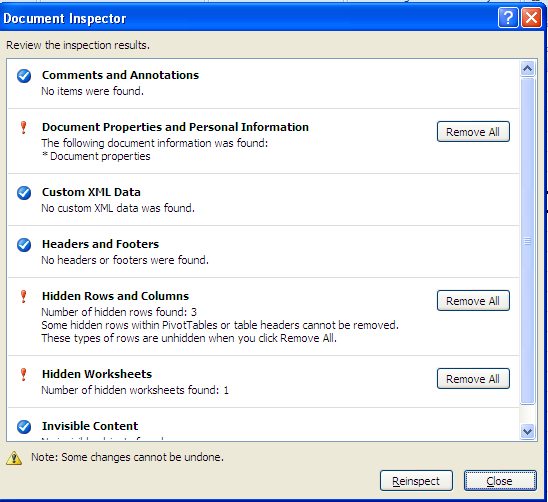
Excel inspect the worksheet and returns with its findings. In this case, it found 3 hidden rows and 1 hidden worksheet.

You then have the option of removing what Excel has found.

Disappointingly,the Inspect Document feature did not find  my invisible cell, (I changed the cell font color to white, so that the cell was invisible being white font on white background.); however, I think you will still find it useful.

The Document Inspector is also in Word and PowerPoint.

Converting Text with a trailing CR to a Number

,Don't you just hate it when you import data and see the dreaded CR at the end of a number. You know that Excel automatically treats any cell content as text if it is a mix of numbers and text. This of course is a huge problem if you need to actually use that cell value in a calculation.  Below is a way to convert the content by using the LEN function and the LEFT function.

• The LEN sounds like a useless function but it actually very powerful - it counts the number of characters in a cell =LEN(text). 
• LEFT is a text function and it extracts the specified number of characters =LEFT(text, number of characters).

The LEN function counts the number of characters in the cell and the LEFT function tells Excel to extract everything except for the last 2 characters in that cell. I then multiplied it by -1 to make it negative.

So, in the example above, if you break it down, Excel looks at the LEN (A20)-2 and evaluates that as 5-2 which of course is 3 so now it would read =LEFT(A20,3)*-1. Excel would treat that as =100*-1 and the resulting answer would be -100.