An Accounting Game!

For all you CPAs on the East Coast who are suffering through the blizzard and looking for something to do - check this out.

Free accounting game.  Yes- an accounting game!
So, if you are sitting at home looking out the window at the piles and piles of snow ( or sitting in an airport!) , give this a try. Something to do.  Actually it has been around for awhile and I have a link on my site to it but it's late on Friday and this is all I could come up with.

Check out http://www.revenuerecognitionchallenge.com/
a free online accounting game. Yes- that's right... free accounting game . If you report different revenue types correctly as unexpected scenarios occur and pass the "Schmarbanes-Schmoxley"audit, your stock price goes up and fireworks go off!


It's fun in a nerdy way... what I can say!
Have a good weekend and stay warm.

Cumulative Totals

Sometimes it is the easy stuff that escapes us.
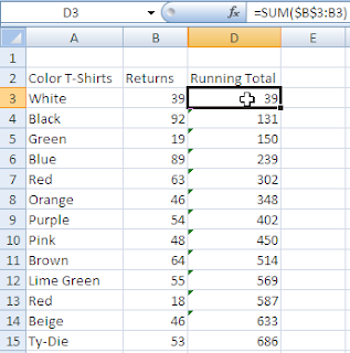
Below is a screenshot showing how to create a cumulative total.

In the example below, I want to create a Running Total and track my T-Shirt Returns.

• Click in cell D3 and type =SUM($B$3.B3)
• Press Enter
• Copy the formula down.

Why this works:                                                                            
The $B$3 creates an absolute cell reference so that as the formula is copied down, it always goes back and refers to B3.
If you click in cell D4, after you create the formula, you would see that the formula has now changed to
=SUM($B$3:B4). The first cell reference is an absolute and anchors the cell reference in place but the second cell reference moves down a row.
The formula at D15 would of course read as =SUM($B$3:B15).

View Multiple Worksheets in the Same Workbook

SEE MULTIPLE WORKSHEETS IN THE SAME WORKBOOK AT ONCE

Frequently people like to look at more than one worksheet in their workbook and flipping back and forth can be bothersome.

So, if you want to view 2 or more worksheets at the same time on your computer screen all you have to do is open a second window.

Select the View Tab and then in the Window group, click New Window.
It doesn’t look like anything happens when you do this however if you look up at the title bar, you will now see a :2 after the file name to show that a second copy (window) has been made.
You can then use each window to display and edit different parts of the same workbook.

The files are mirror images of each other and any change is actually appearing in both at the same time.


Tip: Close out the :2 version first and then you will see the :1 disappear from the original. If you close out the :1 first, it is not a big deal, however you will always have that :2 after the name and then you are always wondering whatever happened to Version 1. :)

Smart Tables in Excel 2007

Excel 2007 offers a wonderful feature that not many people are aware of.  It is called a Smart Table and, in my mind, is basically an advanced version of Excel 2003’s List feature.

Excel considers a list or table to consist of data that is adjacent and does not contain a totally empty column or a totally empty row.
With the Table feature, you can have new data formatted as you enter it, shade alternate rows, instantly sum up the right column and quickly name the table.



The most exciting feature however is that tables are dynamic. As you add or delete data, Excel automatically updates and formats the table. So, what does this really mean for you? It means that if you base a chart, a pivot table or a formula on a table, as data changes in the table, it will automatically update the chart or whatever it is based on. This ensures that you are working with the most current data.


CREATE A TABLE
To create an Excel table

• Type your data into the worksheet as you normally would
• Make sure that you include column headings
• Do not leave any empty rows or columns
• Click in the data and press CTRL+T.

The Create Table dialog box will pop up so that you can double-check the data range and to ensure there is a checkmark in My Table has headers.

• Click OK.

The table feature automatically bands and shades every second row and it applies filter arrows to the column headings. A definite timesaver.
 

 
 
 
 
 
When the table is created, a contextual toolbar also appears.
It allows you, among other things, to quickly sum a column, name the table, change formatting styles as well as remove duplicates.
 
 

Adding data into the spreadsheet is not any different than what you have done before – you simply select a cell in the row immediately below the last row and type the value in.

-If you enter a formula in the adjacent column, Excel will automatically copy it down the entire table and format it.
-If you enter data in the adjacent row, Excel will automatically format it so that it matches the table.


To me, the exciting part of the table is that when you add the total row, Excel automatically calculates the values in the rightmost column. You can change that summary operation or add a total to another column easily.



To Create a Total Row
-Make sure your cursor is in the table
-Click on the Design tab under the new Table Tools tab
-Click Total Row

The last row of your total now displays the sum of the right most column.

Creating and Using a Template

Templates

 

Templates are a useful tool that are often forgotten or overlooked. People use them in Word to create invoices and other standardized forms but never think to apply that standardization to their Excel workbooks.

• If you use custom formats or find yourself applying a standardized formatting to every Excel document that you create (be it fonts, column widths, number formats )then you should consider creating a template.
• It can also be useful if you are working with others on a project such as a budget and want to ensure that the setup and formatting are all the same. You can create a template and then distribute it.

The easiest way to create a template is to simply create a worksheet with the formatting, column widths etc. that you want to use as the foundation and then save it.

 

• Create a worksheet and set it up as you want
• Go to the Office Button
• Select Save As
• Click on the drop-down arrow beside Save As Type
• Select Excel Template or Macro-Enabled Template if your workbook contains macros
• Enter a name for the template
• Click Save
  

 

 

The default is that the template is saved inside the Template Folder. However, you can save it elsewhere.

 ============================================

If you have saved it in the default Template folder, it is extremely easy to retrieve.

Simply click on the Office ButtonSelect New
Select My templates... from the left column

 

 

 

 

 

 

 

 

 

 

 

Select the template you want and click OK

 

 

 

 

 

Since you saved the file as a Template, after you complete work on it and go to save it, Excel will prompt you to name it something else so that the template is not overwritten.