Large Function

I have been playing around with all kinds of functions and arrays. It's a geek fest!

Let's start with a simple Function that can be really useful - LARGE.

The Large function searches through a range of cells and returns the largest value or the 2nd largest or 3rd largest..... whatever you specify.

In this example, Excel goes through the range in B4 through B11 and returns the highest value which is 800. If the formula had read =LARGE(B4:B11,2) then the resulting answer would be 500 as that is the 2nd highest number. Quick way to retrieve something.

And of course, Microsoft thinks of everything so the function SMALL does the exact opposite.

Using Functions Together

5 TExt functions and Date Function Combined......Whew

I am putting together an 8 hour Functions seminar for the Indianapolis CPA Society and I think I am going to restruture it a bit. Usually when function are taught, they are taught as isolated examples. However, a lot of times you really need to use multiple functions together. So, I am going to show some useful examples that people can actually use. I am jumping the gun a bit here but I just put together a useful example and thought I would share it with you.


Frequently dates don't import the way you wish and you need to do a little 'surgery' on them. In the example below, I needed to use 4 Text Functions and 1 Date function. Now, obviously the first time or two you do this, it'll take awhile but then it will be second nature......... well maybe :)

In this example, dates that were imported into Column A are not in a date format familiar to Excel.
Using 5 different functions: 4 Text functions and 1 Date function we can extract, combine and then display Column A values in a date format.










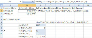
I have broken it apart so that you can identify all the different functions.
The Left function retrieves the 4 leftmost characters in the cell
The Find function searches for the period in the cell and determines that there are 4 characters to get to the period plus 1 = 5 characters
The Mid function goes to the cell and uses the 5 characters + 1 character as the starting point and then grabs the 2 next characters
The Right function grabs the last 2 characters to the rightAll the functions are housed within the Date function which then provides joins the characters together in a familiar date format.
Stayed tuned... let's see what else I can come up with.
If you use any useful combination of functions please let me know. I love to use practical examples.

View 2 Sheets in the Same File at the Same Time

Sorry- I guess you could tell that I took a few days off... I was enjoying sun and wonderful weather on the Massachusetts coast.
Here is a picture of Rockport Harbor.. absolutely beautiful..

Today's topic is Viewing 2 Excel Worksheets in the Same File at the Same Time (that's a mouthful isn't it).

Lotus allowed you to do a 3D perspective oh..so many years ago and while Excel does not have a specific command to view 2 or more sheets in the same file at the same time, it can still be done.

The easiest way to view2 or more worksheets at the same time on your computer screen is to open a second window. To do this select the View Tab and then in the Window group, click New Window. It doesn’t look like anything happens when you do this however if you look up at the title bar, you will now see a :2 after the file name to show that a second copy (window) has been made. You can then use each window to display and edit different parts of the same workbook. The files are mirror images of each other and any changes is actually appearing in both at the same time.

I recommend that you close out the window:2 first. If you don't you will end up with a file named :2 which will drive you crazy over time as you can't get rid of the :2.

That's all for today. Have a great week.

Sorry I haven't updated this in awhile but I will get better. Today, I wanted to talk about grouping sheets together as people start to think about budgets and forecasts for next year.

Grouping is interesting because Excel never talks about it and if you go into Help to read about Grouping it talks about Group and Outline which is a totally different feature. In other words, unless you tripped over it or someone told you about it- you probably have never heard of it.

Quite simply, it allows you to select sheets and anything that you type, format etc on one sheet is automatically replicated on other sheets. It is a great timesaver.

Grouping Sheets
Getting ready to create budgets for 10 departments? Don’t create a budget and then copy it 10 times – instead use grouping. Not only is it faster- it also ensures all your original formatting is retained. Other uses for grouping include printing. Perhaps you want to print Sheet 2, 5 and 6 – the easy way to print them all at once is to group the sheets and then select print. Another use for Grouping is to apply headers and footers to all your sheets at the same time.

Methods for Efficiently Updating/Moving Data Grouping Sheets
Grouping sheets allows you eliminate the need of copying cells in a worksheet to another and then reformatting. Data entered into a group of worksheets is actually placed into each of the worksheets. Any formatting is also included. This feature is particularly useful if you need to have similar worksheets set up in the same format.

To group sheets adjacent sheets:
1. Select the first sheet.
2. Press Shift and hold it down.
3. Click on the last contiguous sheet in the group.
The title bar now shows the word Group after the book name and that all the sheets in the group are active.

Anything that you type on one of the group sheets will automatically be copied simultaneously onto all of the sheets in the selected group including formatting techniques such as changing column widths. Remember to ungroup the sheets when finished so that you can individualize them.

--Use the CTRL key if you are selecting non-adjacent sheets

Deselect Tab
To deselect an individual worksheet, press CTRL + the specific tab.

Ungroup
To ungroup the sheets, select a worksheet tab that was not in the group. You can also right-click and select Ungroup.

Have fun and remember you can ungroup them- make changes and then group them again.

Range Names at Worksheet Level

Range Names at Worksheet Level

I was putting together some information on range names and realized that when I posted my information on range names (under Basic Tips) that I neglected to mention a new feature in Excel 2007.
If you create a range name using the Name Manager icon, you can specify if the range name should be at the workbook scope (this is the default) or you can specify a specific sheet for that range name to be used on. In other words, in Excel 2007, you can actually use a range name more than once as long as it is at sheet level. If you do create a range name at the sheet level, it is only recognized on that particular sheet.

Click on the Formula Ribbon and then go to Name Manager and click New...
Type in a range name and then click the drop-down arrow beside Scope if you want it to be sheet specific. As I mentioned earlier, the default is workbook level.

In all other versions of Excel, you can only use a range name once in a workbook.