Print Macro

I don't know about you but I am tired of always having to change my spreadsheet to a landscape orientation before printing. Personally, I think Microsoft should have made the default oreientation landscape. Anyway, I have been trying to play around and use macros so I decided to just write a macro to do it for me. This is a simple macro - all it does is change the print orientation to Landscape.

The green is just information for the user and is not part of the actual macro.
To access the Developer tab where all the macro features exist, in Excel 2010, you need to:

• Click on File>Options
• Select Customize Ribbon
• Select Developer
• Click OK

Once you have  the Developer tab visible,

• Copy the code below
• Click on the Visual Basic icon (or press Alt+F11)
• Click Insert>Module
• A blank window will display
• Click Edit>Paste
• You can run it to test it or debug it if you wish
• Click File>Close and Return to Excel
• Click the Macros icon
• From there you can edit it, run it, or click on Options to create a shortcut key.

If you record the steps yoursefl, your code will be a lot longer but it will still work. You could also add in whatever other print features you change all the time. I gave mine a shortcut key of Control+Shift+P but you can give it a key combination that makes sense to you.

Sub Landscape_Printing()

'
' Landscape_Printing Macro
' This macro changes the print setting to landscape.
'
' Application.PrintCommunication = False
With ActiveSheet.PageSetup
.Orientation = xlLandscape
End With
Application.PrintCommunication = True
End Sub

 

Pick From A List

If you are constantly typing something such as a list of employee names or a list of cost center codes consider using the Pick From Drop-Down List. It is very easy to use.

Type your data. In the example below, I typed a series of names...

When I wanted to repeat one that I had previously typed, all I had to do was right-click and select Pick From Drop-Down List. The Drop-Down List displays all the names that I had typed above.

Excel then displays the list of names I had previously typed in alphabetical order. Now I can just click on the one I want and Excel will enter it for me. So, it saves a bit of typing.

And no, I'm sorry- I know what you are thinking  but unfortunately it only works with text.

Data Validation, another feature in Excel, also allows you create a list and is a bit more flexible although this Pick From Drop-Down list is a bit quicker.

USE THE OFFSET FUNCTION TO CREATE A HORIZONTAL CHART THAT AUTOMATICALLY UPDATES

In most cases people tend to add data to a chart vertically however there are instances where you need to add columns of data to your chart. To have the chart automatically pick up additional columns as they are added you should use the OFFSET function.
In the example below I have widget sales for January through March.

 

 
 
 
I wanted to create a chart so that as I added April through December sales into the chart, the chart would automatically include the new data without me having to do anything to the chart.

 

First, I need to create my chart as I normally would. I am using a column chart as i think it is a little easier to see.

 

 

 

 

 
 
 
 
 
 
 
 
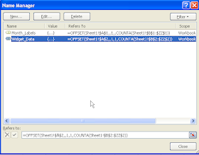
Then I need to identify each of the 2 rows to Excel by creating defined names.
We are going to create a name and formula for the months and then for the widget sales.
Go to the Formula tab and select Define Name

• 
   
• In the Name box type Month_Labels
• In the Refers To box: type =OFFSET(Sheet1!$A$1,,1,,COUNTA(Sheet1!$B$1:$ZZ$1))
• Click OK

This is telling Excel to go to cell A1 and then move over 1 column and to start selecting data all the way to Column ZZ.  Now currently there is only data Columns A through D but as we add additional columns of data, Excel will be looking for it.
Now we need to define the widget sales

• Go to the Formula tab and select Define Name
• In the Name box type Widget_Data
• In the Refers To box: type =OFFSET(Sheet1!$A$2,,1,1,COUNTA(Sheet1!$B$2:$ZZ$2))
• Click OK

This is telling Excel to go to cell A2 and to move over 1 column and select data from B2 through Column ZZ.

 

 

 

Click in the chart and select the data series and replace the cell references to the formula names of Month_Labels and Widget_Data

Now as you add April and May's data, Excel will automatically include it in the chart.

Click here to download the Excel file.