Today, I thought I would talk about the Frequency functions. This was quite useful to me when I taught at Butler. For all you of you instead of grades- consider using it to track warranty information or perhaps returns or HR data such as salary levels in your organization. If you think about it, I am sure you will find a couple of uses for this.
Frequency Distributions
A frequency distribution allows you to measure performance of one item against others. A good example would be a comparison of students in a class and the grade category that they fall into. Again, consider tracking returns of an item by color or even item number. Other possibililies include a breakdown of prices for a product line or even ages or education of your workforce.
A frequency distribution is a table where data in a spreadsheet is counted into bins. It is a good habit double check your calculation - to verify that the number of items in your input range equals the number of observations in your answer. Use a COUNT function on the input range and the sum function on your answer.
To create a frequency distribution
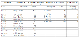
1. Create a set of numbers to use as bins. Keeping with our grading metaphor, you may want to have five (5) bins such as the following: 100, 89, 79, 69 and 59.
In our case, we are asking Excel to group grades so that we can see the number who earned a grade between 100 and 90 as one category (the A group), those who earned a grade between 80 and 89 (the B group) etc. all the way to a count of those who earned a grade between 0 and 59.
The bins created are in Column F. The description was added in Column D and E is solely for clarification and documentation and is not used in the calculation.
2. Select the cells where you want your answer to go. In this case, select G2.G6.
3. Type = Frequency (and then select the input range. In this case you would select C2.C11.
4. Type in a comma and then select your bin range. In this case F2.F6.
5. Type a closing parenthesis. Your formula should look like =frequency (c2.c11, f2.f6)
6. Now the important part - press CTRL+SHIFT+ENTER. The resulting frequency distribution should appear and resemble Column G. The resulting formula should look like {=frequency (c2.c11, f2.f6)}
So, what does this tell you? It tells you that in the A bin which are grades between 90 to 100 (inclusive), 6 people fell into that category whereas only 2 people ended up in the C category which was from 70 to 79 inclusive.
A couple of comments:
Excel puts the brackets around the formula to show that it is an array. If at step 2, you only selected G2 and after going through the other steps, you copied the formula down- the answer would be wrong, Because this is essentially an array formula, you need to select all the cells G2.G6 at one time for this to work.
Also, bins must be numeric. In the example below, I want to figure out how many people have less than a high school education but my data and the bins must be numeric. Again, the description is purely for the user- it is not used in the calculation. As mentioned above, it is a good idea to sum your Frequency and then count your observations to make sure that the number are the same. In the example below, my frequencies total 40. If I counted the number of people in my data, it should total 40 people otherwise there is a problem somewhere.


No comments:
Post a Comment