Excel 2010 Overview

I sat in this morning on a webinar that overviewed Excel 2010. Seems like we just started with Excel 2007 doesn't it? The webinar was very informative and I thought some of you might be interested in the high points. I need to thank Chandoo for posting information on the webinar.

• First, I know everyone will be thrilled to hear that the File Menu is making a comeback! The Office button disappears and is replaced with  a File tab. Hurray.
• Microsoft has also enhanced it. For example, now you can "stick" files that you want to always display when opening Excel.
• Second, the ribbon is customizable so that you can add your own tabs and then groups within the tabs.
• Paste Preview will now display the different versions of what will actually paste: values..formulas etc .
• Microsoft is adding in a screenshot feature so that you can take a picture of part of your spreadsheet

New Features include:
Sparklines
 - Mini charts - This is an exciting feature for those of you creating dashboards.
Slices
 - think of Slices as mini dialog boxes that appear on the screen so that you don't have to keep clicking        drop-down menus in your pivot table
PowerPivot Addin that will be useful for people connecting to large databases to pull their data
Solver User Interface

Other features have been enhanced to some degree and these include Conditional Formatting, Tables, Pivot Table Options (easier to do calculations) as well as Filtering and Macro Recording.

To learn more about these features and/or to download Office 2010 Beta (it expires in October 2010), click here.   Chandoo's website is previewing in detail a lot of the new features so you may want to take a look there too. Click here to get to his articles on 2010.


I wasn't too excited about Excel 2007 but I have to say I am looking forward to using Excel 2010. I'm hoping they "fixed" some of the 2007 Chart features but I fear not.  I mean after all they need something to work on for Excel 2012 or Excel 2013.

Have a good day.

INDIRECT FUNCTION

The INDIRECT function is cool. When you first look at it, you wonder what the heck you can do with it and then all of a sudden you realize that you have a lot of applications for it.
The INDIRECT function accepts a text string as an argument and then evaluates the text string to determine the relevant cell or range reference. What does that mean?
Let's start with a basic example:


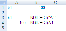
Based on the Excel spreadsheet screenshot:
=Indirect(”A1") Returns the contents of the referenced cell which is B1

=Indirect(A1) Returns the actual contents of the referenced cell. Excel sees that cell A1 contains the cell reference B1 and goes and returns the value in B1 which is 100.
If cell A1 had contained text such as CPA, then CPA would have been returned if quotes had been used.
However, if quotes were not used you would see a #REF! Error since there is no cell reference called CPA.

Okay, so what can you really do with this? Does anyone have an Excel workbook that has a sheet for each month and a summary sheet that displays key calculations for the current month? If not, perhaps you have a file contains sheets by brand or product line and then a summary sheet? If so then you probably spend a lot of time linking or copying and pasting. Using the Indirect function will save you time and allow you to more time to analyze the data.


In the example below, I have a summary sheet that tracks the current month volume in both dollars.

The supporting sheets with the store information are labeled by month - Jan, Feb and March.

 Instead of linking or pasting numbers into summary sheet cells B6 each month I can automate the process by using the Indirect function. Notice that cell B4 is the cell showing the month’s key values that I am displaying. In this case January.

 The formula I use to retrieve the total shipment dollars shipped in January is

This formula tells Excel go look at cell B4 and to find the cell or range reference found there. In this case Excel looks for JAN which is a sheet name. The ampersand joins the month name with the cell reference of G19. Excel goes to the January sheet and returns the value found in G19 to this summary sheet. If I wanted to see the value of G19 on the February sheet all I have to do is change the name in B4 to Feb to match the name of the actual sheet.

Excel goes over to the Jan sheet and then retrieves the value of 2,556,375 at cell G19 and returns it to the summary sheet.







This example was a bit simple – what happens if every month has a different number of rows or isn’t nicely totaled? If the column had not been totaled I could have used a formula such as this

or if you had no idea how many rows were being populated you could have substituted G:G for G1:G40.
To make it more efficient, use a data validation drop-down list of months in B4.

A new use for F9

I hope you all had a great weekend.  My Mother's Day was excellent- in case you were wondering. Too cold to play golf so my daughter and I shopped. Fun either way.

Most people know that the F9 key allows you to recalculate your spreadsheet and can be quite useful if you have turned off automatic recalculation due to the size and/or complexity of your worksheets. If you are not familiar with it, F9 recalculates the entire file whereas Shift +F9 recalculates the current sheet.

However, this weekend I learned a new use for it from a fellow Linked-In member that I thought you might be interested in it.

If you highlight a formula or function in the formula bar and press F9, Excel will substitute that element within the formula with the result. For example, assume the sum of A1 through A10 is a value of 20. If you created the formula =SUM(A1.A10)+1 and highlighted =SUM(A1.A10) in the formula bar and then pressed F9, Excel would display 20 on the formula bar. Press F9 again, and it will revert to the calculation.
You need to select the formula name =SUM, not just the cell references.

This is a bit quicker than going to the Formula Auditing group on the Data Ribbon and selecting Evaluate Formulas.

Have a great Monday.

Basic Chart and Table Design IQ Quiz

Stephen Few, author of Information Dashboard Design, offers some great insights on how to be visually intelligent. 

 No matter where you are in your business life - the company's "chart guy",  the occasional presenter or just learning about charts and tables, you will appreciate this GraphDesign IQquiz.

The point it makes is loud and clear and everyone should find it useful.

 I am happy to say that I scored 10 out of 10.  So, what's your score?

Check it out when you have a moment

http://www.perceptualedge.com/files/GraphDesignIQ.html

Have a great Mother's Day. I'm looking forward to a fun day of brunch, golf with my daughter and dinner with my family. I hope that your day is equally good.

Cheers.

Patricia

NESTED IF STATEMENTS

Nested IFs are one of those "must knows" and I couldn't believe that I had not written about it before.
A nested IF is an IF statement that has been placed within another IF. This is very handy if you want to test more than 2 conditions.

In Excel 2003, you can have a maximum of 7 levels of IF statements within an If statement although I have had people tell me they have created nested IFs with more than 7 levels using range names. In Excel 2007, you can have up to 64 levels.  Before we go any further, let me just say, that if you are anywhere over 7, you seriously need to learn about VLOOKUPs and INDEX MATCH functions. Honestly, no one wants to try to untangle or edit a 64 level IF statement.

Let's use this scenario: A bike company is offering some promotional tours and is trying to keep track of  them. There are 3 alternative statuses- the tour is underbooked, overbooked or full.

To create a nested IF with three conditions……………

Start the IF as you normally would and enter the test/condition and the True argument. In the example, I clicked in E14 and then clicked on the fx button to get the IF dialog box.

I typed =IF(C14 is greater than D14 as the Test and then clicked in the Value if True section and typed "underbooked"
(the quotations are because it is text)

Okay - I have taken care of one scenario- underbooked.

Then I clicked in the Value if False section (make sure you are in the False section!)
and  then clicked on the drop-down arrow in the Name box (above column A) and selected IF

The current dialog box collapses and is replaced with a brand new IF dialog box. (Don't worry -if you check the formula bar, you will see the earlier part of the formula still exists!)
I have 2 tests left since I have already taken care of the underbooked status.

 So, in the Logical Test, I tested C14=D14 and in the Value if true section typed "Full".
 "Overbooked" goes in the Value if False by default since that is the only option left.

If you click back on the fx button, Excel will bring back the entire nested IF so that you can see how it looks. Excel tests the first condition and if the test it met, it stops. If the test is not met, it continues to the next test and so on. 
In this particular example, the order of the tests did not matter, however if you are testing years or numbers, it may.
My rule of thumb is to start at the highest or largest number and work your way down.

Frequency Distribution

I hope you all are enjoying this great weather. I've been working away preparing for a couple of seminars that I am doing in May and I have to tell you I've been having a blast learning all kinds of new tricks and tips that I will be sharing shortly with you. 

Today, I thought I would talk about the Frequency functions. This was quite useful to me when I taught at Butler. For all you of you instead of grades- consider using it to track warranty information or perhaps returns or HR data such as salary levels in your organization. If you think about it, I am sure you will find a couple of uses for this.

Frequency Distributions


A frequency distribution allows you to measure performance of one item against others. A good example would be a comparison of students in a class and the grade category that they fall into. Again, consider tracking returns of an item by color or even item number. Other possibililies include a breakdown of prices for a product line or even ages or education of your workforce.
A frequency distribution is a table where data in a spreadsheet is counted into bins. It is a good habit  double check your calculation - to verify that the number of items in your input range equals the number of observations in your answer. Use a COUNT function on the input range and the sum function on your answer.

To create a frequency distribution

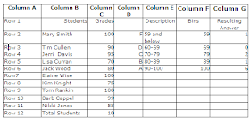
1. Create a set of numbers to use as bins. Keeping with our grading metaphor, you may want to have five (5) bins such as the following: 100, 89, 79, 69 and 59.

In our case, we are asking Excel to group grades so that we can see the number who earned a grade between 100 and 90 as one category (the A group), those who earned a grade between 80 and 89 (the B group) etc. all the way to a count of those who earned a grade between 0 and 59.

The bins created are in Column F. The description was added in Column D and E is solely for clarification and documentation and is not used in the calculation.

2. Select the cells where you want your answer to go. In this case, select G2.G6.

3. Type = Frequency (and then select the input range. In this case you would select C2.C11.

4. Type in a comma and then select your bin range. In this case F2.F6.

5. Type a closing parenthesis. Your formula should look like =frequency (c2.c11, f2.f6)

6. Now the important part - press CTRL+SHIFT+ENTER. The resulting frequency distribution should appear and resemble Column G. The resulting formula should look like {=frequency (c2.c11, f2.f6)}

So, what does this tell you? It tells you that in the A bin which are grades between 90 to 100 (inclusive), 6 people fell into that category whereas only 2 people ended up in the C category which was from 70 to 79 inclusive.
A couple of comments:
Excel puts the brackets around the formula to show that it is an array. If at step 2, you only selected G2 and after going through the other steps, you copied the formula down- the answer would be wrong, Because this is essentially an array formula, you need to select all the cells G2.G6 at one time for this to work.

Also, bins must be numeric. In the example below, I want to figure out how many people have less than a high school education but my data and the bins must be numeric. Again, the description is purely for the user- it is not used in the calculation. As mentioned above, it is a good idea to sum your Frequency and then count your observations to make sure that the number are the same.  In the example below, my frequencies total 40. If I counted the number of people in my data, it should total 40 people otherwise there is a problem somewhere.