Information Functions - ISERROR and others

Information functions
ISBLANK, ISNUMBERand ISTEXTas well as ISERROR are information functions and are usually found nested in other functions such as an IF since they do little by themselves. The three functions return either a True or False, which can be used in other calculations to continue a calculation or decision.

When you first look at Information functions, you wonder - why bother. However, if you import a lot of data you may find them useful. And if you nest an information function within an IF Function then it can be very powerful.

Below are a couple of the more useful Information functions. By themselves, they test a cell and return a result of either True or False

The ISBLANK function tests whether a cell is empty and returns a value of TRUE if it is empty. =ISBLANK (cell reference)

The ISNUMBER function tests a cell's value to determine if it is a number. If the contents of the cell are a number then it is true
otherwise it is false. =ISNUMBER (cell reference)

ISTEXT tests whether the contents of the cell are text and return true.
=ISTEXT (cell reference)

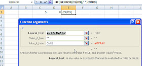
The most common use is combining =ISERROR() with an IF to replace errors in cells with a blank. The IFERROR() function that is available in Excel 2007 reduces the need for this but if you have Excel 2003 you definitely need this.

Below is an example, the ISERROR checks to see if cell the formula C9/D9 will result in an error. If this is TRUE, then the error is replaced with a blank cell - otherwise it is FALSE and the result of C9/D9 is displayed in the cell.

When using an Information function with an IF Function:

Put the TRUE and FALSE components in first and then enter the information into the test last otherwise the dialog box collapses on you and have to manually type in the formulas. This is particularly true of Excel 2003.

Counting

Count Functions

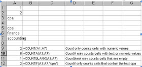
Who knew that there were so many count functions? I have found that a lot of people don't understand that =COUNT() only counts numbers. There are a number of different count functions. So, here goes...........

=Count()
Counts the number of cells that contain numbers and numbers within the list of arguments. Use COUNT to get the number of entries in a number field in a range or array of numbers.

=CountA()
Counts the number of cells that are not empty and the values within the list of arguments. Use COUNTA to count the number of cells that contain data in a range or array.
In the following example,

=CountBlank()
Counts empty cells in a specified range of cells.Excel does not consider it a blank cell if there is a space in the cell (someone pressed the spacebar in the cell)

=CountIF() and =CountIFs()
Counts the number of cells within a range that meet the given criteria.

Don’t forget that you can use wildcards with COUNTIF and COUNTIFs.
For example, =countif (A1:A7,”*P*”) would return a value of 2 as it would count only the words that contained a P.

Database Functions

DATABASE FUNCTIONS

Sorry- I just finished baking an apple pie so I decided to use it as my example.

Database functions operate similar to other Excel functions.

These database functions can be very effective and could easily be used in lieu of sumif or countif if you have Excel 2003 and even Sumifs and Countifs in Excel 2007.

The syntax is =FieldName (database range, field, criteria).
The database range is the entire range of data including headings.
The field is the column that you wish to perform the function on.
The criterion is the range of cells that you are testing to see if they meet specific conditions.

Some of the more common Database Functions are:

=DSUM (database range, field, criteria)
=DCOUNT (database range, field, criteria)
=DAVERAGE (database range, field, criteria)

To use Database functions you need to have set up a separate criteria area either above or below your data where you specify what you are testing for.

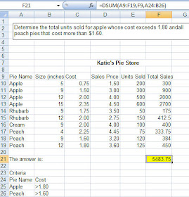
Below is an example of how the DSUM function would be used. Here my database range is A9.F19, which includes your headings.

I want it to sum up Total Sales which is in Column F so my field is F9.

My criteria is at rows A24.B26 and specifies all Apple pies have a cost exceeding $1.80 and all Peach pies that have a cost exceeding $1.60.

So, =DSUM(A9:F19, F9,A24.B26) is saying add up Total Sales for all apple pies that have a cost greater than $1.80 and all peach pies that have a cost greater than $1.60

It is important to remember that the headings on the criteria at row A24 exactly match the column headings at row 9 so you may want to copy them to make sure they are set up the same.

It is also important to understand that Excel reads each row of the criteria as an OR statement.

(My data does not have to be organized by pie name- I just did that so it was easier for you to see.)

IF_Error Function

Sorry- I have just been swamped. between finding pilots to pilot my self-study CPE courses, writing Excel courses and lecturing but I want to keep this up to date.

Today, we are going to cover IF_ERROR which is a new function in Excel 2007. If you are more of a visual person - at the bottom of the blog is a video of IF_ERROR.

Cleaning up Error Messages
The good news is that Excel 2007 has made it easy to get rid of error messages with a new function called IFErrror.
The syntax for IFError is =(value,value_if_error).
In the example below, an error message was created because the customer at row 3 had 0 sales last year as compared to current year. The equation used was =(C3-B2)/B2 to determine the percentage increase from the prior year.

Tip: Anything inside quotation marks is treated as a literal. So. “ “ is interpreted as a blank space. If the function had read =IFERROR((c2-B2)/B2,”Not Applicable” then the text Not Applicable would have printed in cell D3 instead of a blank space.

Have a great weekend - fall is definitely here!

Rounding Functions

Round and Round she goes................
I didn't realize how many different rounding functions there are. And, I assuming neither did you.
=Round, =Roundup() and =Rounddown() all round a number to a specified number of decimal places.
=Round(12,3456,1) returns a value of 12.3 since 1 decimal place was specified.
=Round(12.3456,2) return a value of 12.35 since 2 decimal places were specified.

RoundUp always rounds away from the Zero and RoundDown always rounds toward the Zero.
=Roundup(12.3456,1) returns a value of 12.4
=Rounddown(12.3456,1) returns a value of 12.3

Rounding to a Multiple
MRound(), Ceiling() and Floor() round numbers to a specified multiple.
These 3 functions can be used for rounding price points or time.

=MROUND($12.94,5) will round it to the nearest 5 increment and display as $12.95
=MRound($12.94,.025) will round to the nearest .25 increment and display as $13.00


Ceiling() and Floor() are traditionally used with dollar values. They will not round if the number is already a multiple of the number. For example, =Ceiling(3.4,1) will still display as 3.4 since 3.4 is already a multiple of 1.

Evaluate Formulas in Excel

Since we are talking about functions I thought I would mention the Evaluate Formula feature in Excel. You can see the different parts of a nested formula evaluated in the order the formula is calculated.


This is really useful for nested IF statements and other complex calculations



Select the cell you want to evaluate.
Only one cell can be evaluated at a time.

• Click the Formula tab
• Select Evaluate Formula to examine the value of the underlined reference. The result of the evaluation is shown in italics.
  If the underlined part of the formula is a reference to another formula, click Step In to display the other formula in the Evaluation box. Click Step Out to go back to the previous cell and formula.
  Continue until each part of the formula has been evaluated.

To see the evaluation again, click Restart.
To end the evaluation, click Close.