I sure did - started the weekend out at the Naked Chopstix which has the best sushi ever. If you ever make it there, make sure to try the Maui roll! Ended the weekend at the Indiana State Fair eating kettlecorn and walking and walking. Along with the typical fair stuff, we saw a dog agility show, a car show and finished up with a demolition derby that my daughter loved. My favorite part was the car show where I saw my dream car - a 1958 Corvette - a beauty.
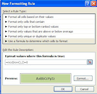
Anyway, let's talk about conditional formatting and applying rules. As I mentioned in my last post there is a lot you can do with conditional formatting and a lot of it is pretty easy to figure out but I thought it would be worthwhile to chat about using formulas and rules. Below are the steps you can use to apply a rule to data. In my example here I am using the MOD function and telling Excel to shade every second row of my P&L so that it is easier to read. I am specifying 2 in the MOD function so that every second row is shaded and I am specifying green as that is the traditional accounting color but obviously you can select any color you want - just make sure that it is light enough that that the data can be seen through it.
1. Select your data

2. Click Conditional Formatting on the Home Ribbon.
3. Select New Rule.
4. Click on Use a Formula to determine which cells to format.
5. In the rule description, type =MOD(row(),2)=0.
6. Click Format
7. Select a light green fill.
8. Click OK.
9. Click OK.
And voila.. it should look something like my example below:


No comments:
Post a Comment